Cones
Light Detection: Rods and Cones
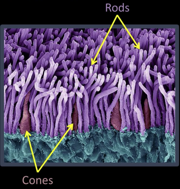
Cones:
- 6-7 million cones in the retina
- Responsible for high-resolution vision
- Discriminate $\color{red}{c}\color{maroon}{o}\color{blue}{l}\color{green}{o}\color{pink}{r}\color{yellow}{s}$
- There are three types of color sensors: $64\%\,\color{red}{\text{ red, }}32\%\color{green}{\text{ green, }}2\%\color{blue}{\text{ blue}}$

Wait!!! I am going to the Camp Nue for FC Barcelona vs Liverpool FC champions league semi-final match. I will be back in a minute
Waaaaaaaaaaaaaaaaaaw. What a game!!!. I am speachless. People asks me are you really going to spend all that money and time to watch a football match, and Messi answers them from the field: I will pay him off every single second and every single penny. Gracias Messi.
Messi scored his 600 goal with Barcelona in the most astonishing way. While I was hesitant at the begining (because it was a long shot), fortunately, I took my mobile out and recorded it
# Uncomment the below code and run to enjoy.
# Comment it out back and run before exiting
# as this might cause the notebook to crash
# in the next time you open it

# from IPython.display import HTML
# HTML("""
# <br/>
# <center><font color="red" size="16px">Messi. Messi. Messi.</font></center>
# <center>
# <video controls width="620" height="440" src="imgs/messi_magic.mov" type="video/mp4">
# </video>
# </center>
# <br/>

# """)
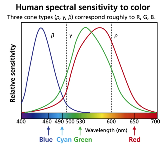
Tristimulus Color Theory

Spectral-response functions of each of the three types of cones
- Can we use them to match any spectral color?
Color Matching Function Based on RGB
Most spectral color can be represented as a positive linear combination of these primary colors(but..)
But some spectral cannot - need to add some red

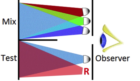

Color is a Psychological Phenomenon
green triggers green cone more than red cone, red triggers red cone more than green cone, when the two cones are balanced, the human vision can't tell the difference

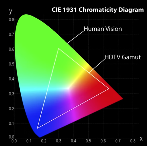
CIE RGB Color Space
Color matching experiments [Wright & Cuild 1920s]
- Mapped physical wavelengths to perceived colors
- Identified relative similarity and difference between colors
- Result: CIE RGB space defined
Color perceivable by the human eye

CIE XYZ color space
A new space with desired properties
- Easy to computer - linear trasform of CIE RGB
- Y: Perceived luminance
- X, Z: Perceived color
- Represents a wide range of colors
$$x = \frac{X}{X+Y+Z}$$
$$y = \frac{Y}{X+Y+Z}$$
CIE $\color{blue}{L*a*b*}$ Color Space
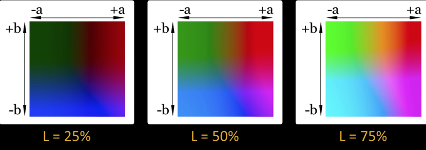
Cylindrical view
Think of chroma (here a,b) defining a planar disc at each luminance level (L)

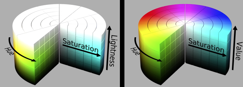
HSL and HSV color space
Quiz
If hue values range in [0, 360], what is the absolute difference between the following pairs of hues?
225 and 75: 150
45 and 315: 90


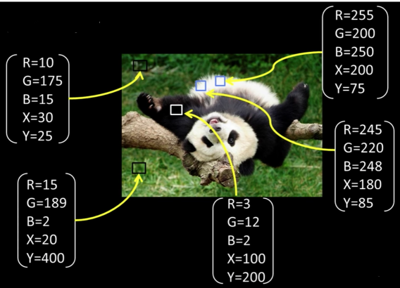
Revisiting Pixels
"Picture element" at location $\color{blue}{(x,y)}$, value or color $\color{blue}{c}$
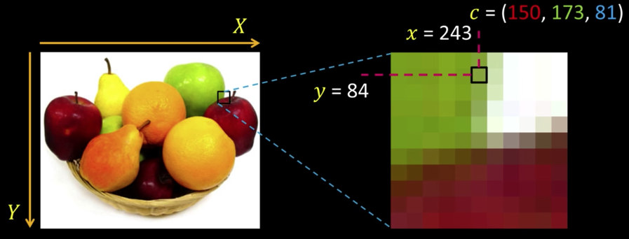
Color values are vectors, here ($\color{red}{R}$, $\color{green}{G}$, $\color{blue}{B}$)
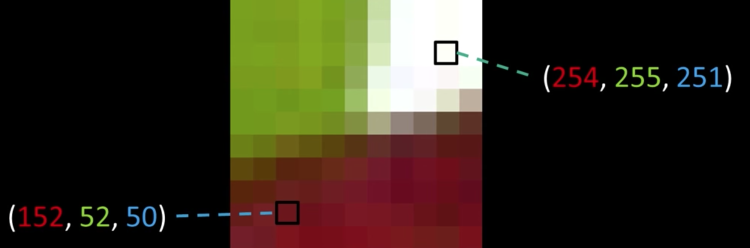
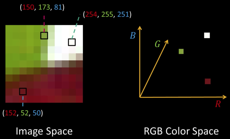

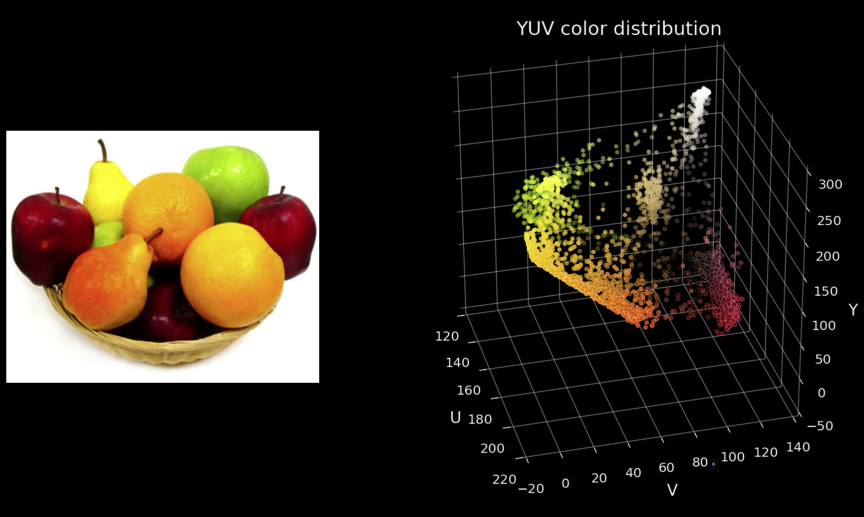
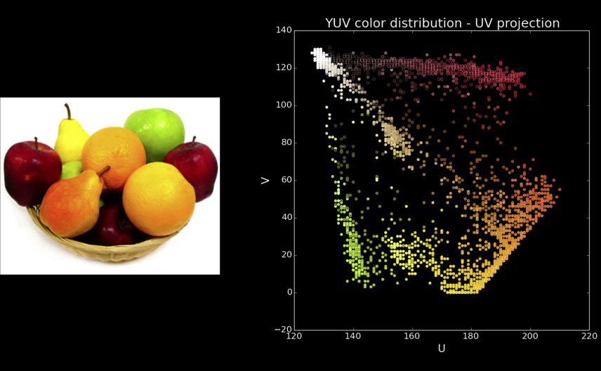
Quiz: Plotting Pixels in a Color Space Quiz
What does this view enable us to do?
- Think about clusters of pixels that are similar in color
- Understand the shape and size of objects present
- Identify pixels that are different, and seperate them
- Count how many pixels of each color there are
%matplotlib inline
import cv2 as cv
import matplotlib.pyplot as plt
import numpy as np
from mpl_toolkits.mplot3d import Axes3D
from IPython.display import clear_output, Image as NoteImage, display
import PIL
from io import BytesIO
def imshow(im,fmt='jpeg'):
    #a = np.uint8(np.clip(im, 0, 255))
    f = BytesIO()
    PIL.Image.fromarray(im).save(f, fmt)
    display(NoteImage(data=f.getvalue()))
def imsave(im,filename,fmt='jpeg'):
    #a = np.uint8(np.clip(im, 0, 255))
    PIL.Image.fromarray(im).save(filename, fmt)
def imread(filename):
    img = cv.imread(filename)
    img = cv.cvtColor(img, cv.COLOR_BGR2RGB)
    return img
def rgb_to_color(rgb):
    return f"#{hex(rgb[0])[2:].zfill(2)}{hex(rgb[1])[2:].zfill(2)}{hex(rgb[2])[2:].zfill(2)}"#f'rgb({rgb[0]}, {rgb[1]}, {rgb[2]})'
def img_to_colors(img):
    return [rgb_to_color(i) for i in img]
def plot_in_rgb_space(img):
    fig, ax = plt.subplots(1, 1, subplot_kw={'projection':'3d', 'aspect':'equal'})
    fig.set_size_inches((20,15))
    c = img_to_colors(img.reshape(-1,3))
    ax.scatter3D(img[:,:,0],img[:,:,1],img[:,:,2],c=c)
img = imread("imgs/L938.png")
imshow(img)
plot_in_rgb_space(img)


def cfilter(img,r,g,b):
    img2 = img.copy()
    img2[(img2[:,:,0] > r) | (img2[:,:,1] > g) | (img2[:,:,2] > b)] = [255,255,255]
    return img2
imshow(cfilter(img,255,50,50))

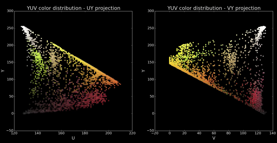
Seperate Intensity and Color
How intensity affects color values
Solution: Seperate intensity and color

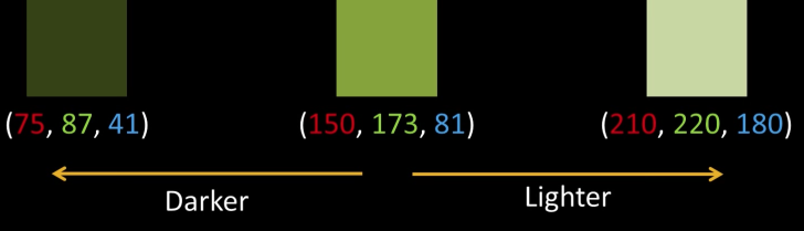
Define intensity ($\color{blue}{Y}$) as some combination of $\color{blue}{R}$,$\color{blue}{G}$,$\color{blue}{B}$
$$\color{blue}{Y = W_R\times R + W_G \times G + W_B \times B}$$
$$\color{blue}{= 0.299\times R + 0.587 \times G + 0.114 \times B}$$
Then compute new color values, taking out intensity
$$\color{blue}{U = U_{max}\frac{B-Y}{1-W_B} \approx 0.392 \times (B-Y)}$$
$$\color{blue}{V = V_{max}\frac{R-Y}{1-W_R} \approx 0.877 \times (R-Y)}$$
Assuming $\color{blue}{R}$,$\color{blue}{G}$,$\color{blue}{B}$ and $\color{blue}{Y}$ are in the range $\color{blue}{[0,1]}$
$$\color{blue}{U \in [-U_{max}, U_{max}]}\color{black}{\text{ and }}\color{blue}{V \in [-V_{max}, V_{max}]}$$

import cv2
import numpy as np
def make_lut_u():
    return np.array([[[i,255-i,0] for i in range(256)]],dtype=np.uint8)
def make_lut_v():
    return np.array([[[0,255-i,i] for i in range(256)]],dtype=np.uint8)


img_yuv = cv2.cvtColor(img, cv2.COLOR_BGR2YUV)
y, u, v = cv2.split(img_yuv)

lut_u, lut_v = make_lut_u(), make_lut_v()

# Convert back to BGR so we can apply the LUT and stack the images
y = cv2.cvtColor(y, cv2.COLOR_GRAY2BGR)
u = cv2.cvtColor(u, cv2.COLOR_GRAY2BGR)
v = cv2.cvtColor(v, cv2.COLOR_GRAY2BGR)
imshow(y)
imshow(u)
imshow(v)


def yuvfilter_cv(yuvimg,ymin,ymax,umin,umax,vmin,vmax):
    i = yuvimg.copy()
    img2[(i[:,:,0] < ymin) | (i[:,:,0] > ymax) | (i[:,:,1] < umin) | (i[:,:,1] > umax) | (i[:,:,2] < vmin) | (i[:,:,2] > vmax)] = [255,255,255]
    return img2
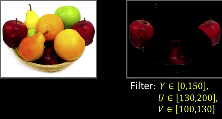
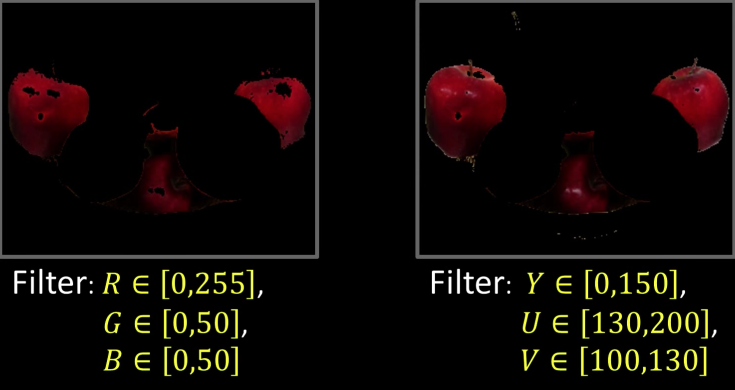
print("RGB Color Filter")
imshow(cfilter(img,255,50,50))
yuv_img = cv2.cvtColor(img, cv2.COLOR_BGR2YUV)
print("YUV Filter")
imshow(yuvfilter_cv(yuv_img,0,150,130,200,100,130))

Intuition and Other Luma Chroma Color Spaces
Why YUV?
- Easier clustering of pixels
- Efficient encoding by Chroma subsampling
- Recall, human vision is more sensitive to intensity changes
- Y channel can now use more bits
- E.g., YUV422 - to represent 2 image pixels, it uses 2 bytes for Y, and 1 byte each for U and V
Other luma-chroma color spaces
- $YC_bC_r/YP_bP_r$ - video transmission, compression
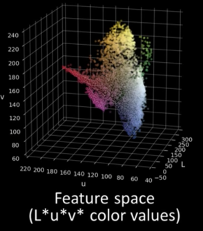
- CIE L*a*b*
- Based on human perception
- Intensity channel: L* = lightness
- Color-opponent: a = red-green, b = blue-yellow
- CIE L*uv* - like L*a*b* but easier to compute
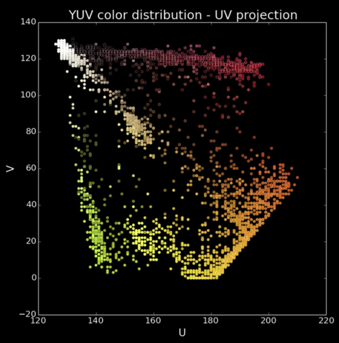
Back to plotting image pixels (Plotting in HSV)

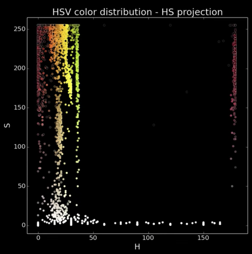
Focus on HS projection
- What do you see?
Colors spread along a single dimension! Hue
A better HS plot
Treat hue as an angle
- Reds from both ends of the spectrum now in proximity
- Better reflects the role of saturation (radius or distance from center)

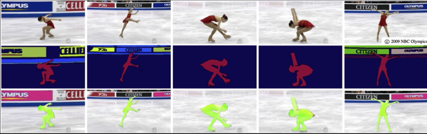
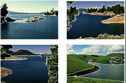
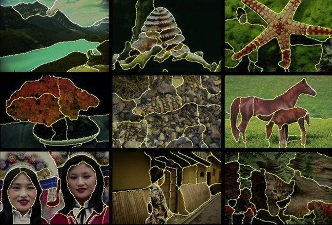
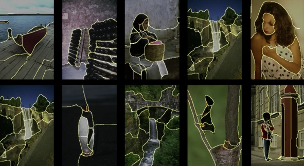
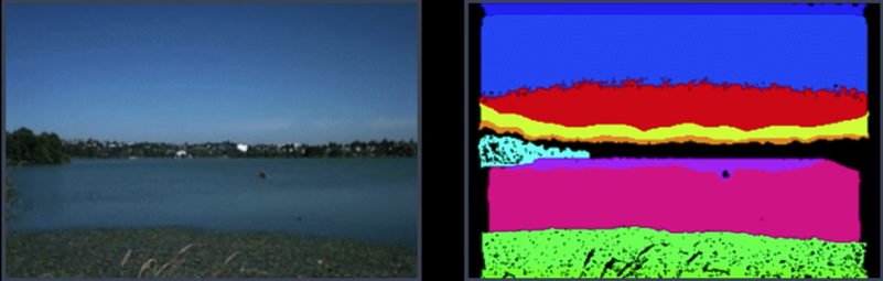
Segmentation of Coherent Regions


Figure Ground Segmentation
- Seperate the forground object (figure) from the background (ground)

Grouping of Similar Neighbors

Extends Beyond Single Images
Clustering
- Goal: choose three "centers" as the representative intensities, and label every pixel according to which of these centers it is nearest to.

- Best cluster centers are those that minimize SSD between all points and their nearest cluster center $c_i$:
$$\color{blue}{SSD = \sum_{cluster\, C_i}\sum_{p \in C_i}||P_j - c_i||^2}$$
- With this objective, it is a "chicken and egg" problem:
- Q: If we know $c_i$'s, how would we determine which points to associate with each cluster center?
- A: for each point p, choose closest $c_i$

- With this objective, it is a "chicken and egg" problem:
- Q: If we knew the cluster membership, how do we get the centers? ?
- A: choose $c_i$ to be the mean of all points in the cluster
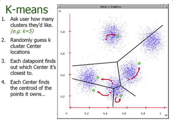
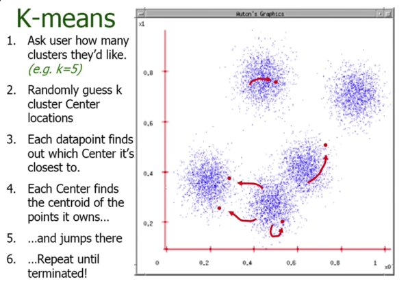
K-means Clustering
- Randomly intialize cluster centers $\color{blue}{c_1,...,c_K}$
- Determine points in each cluster:
- For each point $\color{blue}{p}$, find the closest $\color{blue}{c_i}$; put $\color{blue}{p}$ into cluster $\color{blue}{i}$
- Given points in each cluster, solve for $\color{blue}{c_i}$:
- Set $\color{blue}{c_i}$ to be the mean of points in cluster $\color{blue}{i}$
- If any $\color{blue}{c_i}$ has changed, repeat Step 2
import cv2
import numpy as np
def kmeans(image,segments):
    """
        1. samples : It should be of np.float32 data type, and each feature should be put in a single column.

        2. nclusters(K) : Number of clusters required at end

        3. criteria : It is the iteration termination criteria. When this criteria is satisfied,
                      algorithm iteration stops. Actually, it should be a tuple of 3 parameters.
                      They are ( type, max_iter, epsilon ):

                        3.a - type of termination criteria : It has 3 flags as below:
                                cv2.TERM_CRITERIA_EPS - stop the algorithm iteration if specified accuracy, epsilon, is reached.
                                cv2.TERM_CRITERIA_MAX_ITER - stop the algorithm after the specified number of iterations, max_iter.
                                cv2.TERM_CRITERIA_EPS + cv2.TERM_CRITERIA_MAX_ITER - stop the iteration when any of the above condition is met.

                        3.b - max_iter - An integer specifying maximum number of iterations.

                        3.c - epsilon - Required accuracy

        4. attempts : Flag to specify the number of times the algorithm is executed using different initial labellings.
                      The algorithm returns the labels that yield the best compactness.
                      This compactness is returned as output.
        5. flags : This flag is used to specify how initial centers are taken. Normally two flags are
                  used for this : cv2.KMEANS_PP_CENTERS and cv2.KMEANS_RANDOM_CENTERS.
    """
    image=cv2.GaussianBlur(image,(7,7),0)
    vectorized=image.reshape(-1,3)
    vectorized=np.float32(vectorized)
    criteria=(cv2.TERM_CRITERIA_EPS + cv2.TERM_CRITERIA_MAX_ITER, 10, 1.0)
    ret,label,center=cv2.kmeans(vectorized,segments,None,criteria,10,cv2.KMEANS_RANDOM_CENTERS)
    res = center[label.flatten()]
    segmented_image = res.reshape((image.shape))
    return label.reshape((image.shape[0],image.shape[1])),segmented_image.astype(np.uint8)

def extractComponent(image,label_image,label):
    component=np.zeros(image.shape,np.uint8)
    component[label_image==label]=image[label_image==label]
    return component
def segment(image,segments=3):
    label,result= kmeans(image,segments=segments)
    imshow(result)
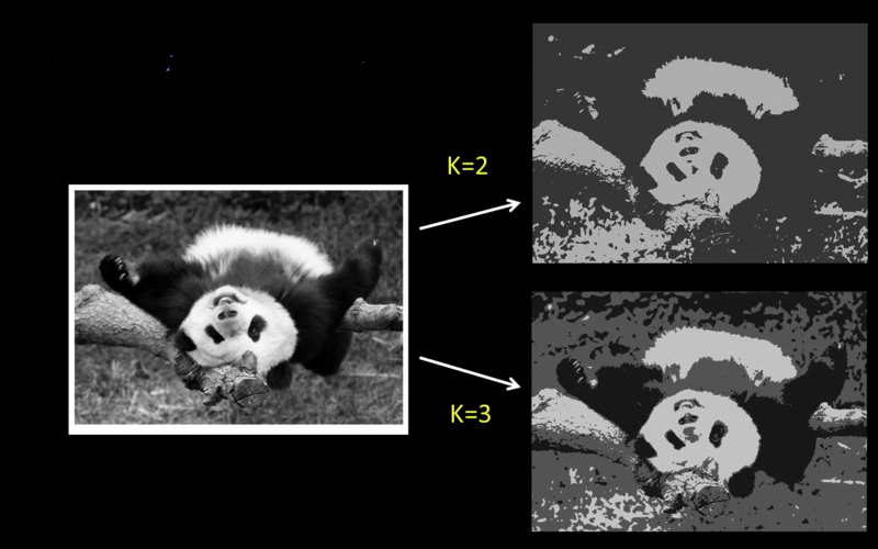
image=imread("imgs/peppers.jpg")
imshow(image)
segment(image,2)


messi = imread("imgs/messi_liverpool.jpg")
imshow(messi)
for i in range(2,20):
    segment(messi,i)


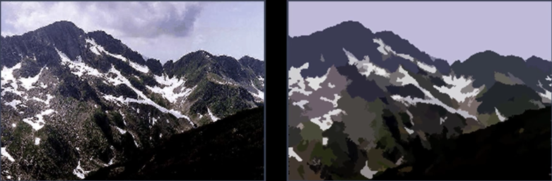
Number of Clusters
Segmentation as clustering
Depending on what we choose as the feature space, we can group pixels in different ways
- Grouping pixels based on intensity similarity


Can be thought of as quantization of the feature space; segmentation label map
Segmentation as Clustering
Depending on what we choose as the feature space, we can group pixels in different ways.
Grouping pixels based on colorsimilarity.

K-means clustering based on intensity or color is essentially vector quantization of the image attributes

Grouping pixels based on intensity+position similarity

Can combine color and location...
Pros and Cons
- Pros
- Very simple method
- Converges to a local minimum of the error function
- Cons
- Memory-intensive
- Need to pick K
- Sensitive to intialization
- Sensitive to outliers
- Only finds "spherical" clusters
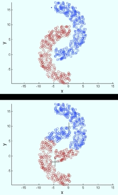
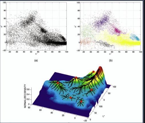
Mean Shift Algorithm
The mean shift algorithm seeks modes or local maxima of density in the feature space


Mean Shift Clustering
- Cluster: all data points in the attraction basin of a mode
- Attraction basin: the region for which all trajectories lead to the same mode

- Find features( color, gradients, texture, etc.)
- Initialize window at individual feature points(pixels)
- Perform mean shift for each window (pixel) until convergence
- Merge windows (pixels) that end up near the same "peak" or mode

## You need to install pymeanshift from https://github.com/fjean/pymeanshift
import cv2
import pymeanshift as pms
original_image = imread("imgs/peppers.jpg")
segmented_image, labels_image, number_regions = pms.segment(original_image, spatial_radius=6,
                                                              range_radius=4.5, min_density=50)
imshow(original_image)
print("Number of segments %d" % number_regions)
imshow(segmented_image)

messi = imread("imgs/messi_liverpool.jpg")
segmented_messi, labels_image, number_regions = pms.segment(messi, spatial_radius=6,
                                                              range_radius=4.5, min_density=50)
imshow(messi)
print("Number of segments %d" % number_regions)
imshow(segmented_messi)

It is so sad... Barcelona lost the second leg against Liverpool FC horribly. They were out of the champions league. Messi showed signs of aging weekness. The hero is dying... The story is about to end

Pros and Cons
Pros:
- Automatically finds basin of attraction
- One parameter choice (window size)
- Does not assume (image) shape on clusters
- Generic technique
- Find multiple modes
Cons:
- Selection of window size
- Does not scale well with dimension of feature space


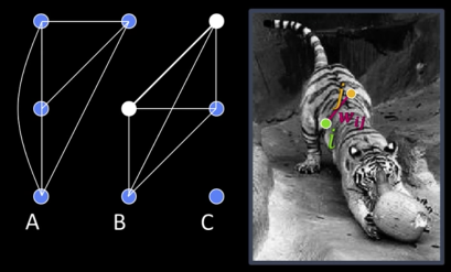
Measuring Affinity
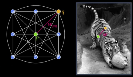
Fully-connected graph
- 1 node (vertex) for every pixel
- A link between every pair of pixels $\color{blue}{<}\color{green}{p}\color{blue}{\text{, }}\color{orange}{q}\color{blue}{>}$
- Affinity weight $\color{maroon}{W_{pq}}$ for each linke (edge)
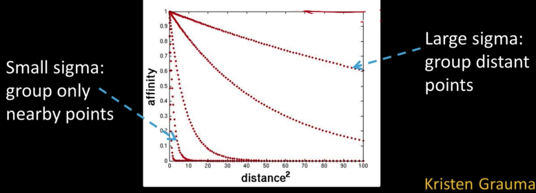
- $\color{maroon}{W_{pq}}$ measures similarity: Inversely proportional to difference (in color and position...)
$$\color{blue}{\text{aff}(x_i,x_j) = exp \left ( -\frac{1}{2\sigma^2}dist(x_i,x_j)^2 \right ) }$$
Segmentation by Graph Partitioning
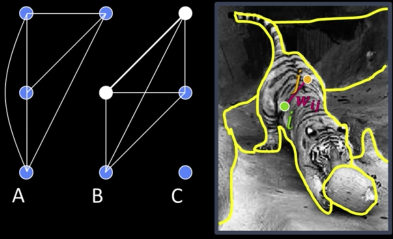
Break Graph into segments
- Delete links that cross between segments
- Easiest to break links with low affinity
Results
- Similar pixels should be in the same segments
- Dissimilar pixels should be in different segments
Graph Cut
$$\color{blue}{cut(A,B) = \sum_{p\in A,q\in B}w_{pq}}$$
Set of edges whose removal makes a graph disconneted
Cost of a cut: Sum of weights of cut edges
A graph cut gives us a segmentaion
- What is a "good" graph cut and how do we fine one?
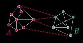
Find minimum cut
- Gives you a segmentation
- Fast min-cut algorithms exist
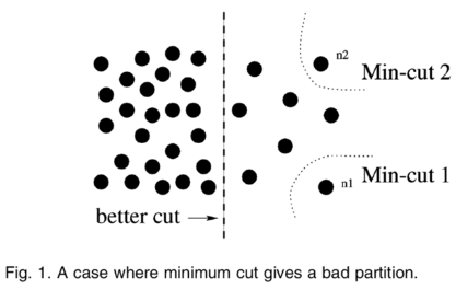
Minimum cut
Problem with min cut:
- Weight of cut proportional to number of edges in the cut
- Tends to produce small, isolated components
Normalized cut
Fix bias of min cut by normalizing for size of segments:
$$\color{blue}{Ncut(A,B) = \frac{cut(A,B)}{assoc(A,V)} + \frac{cut(A,B)}{assoc(B,V)}}$$
$\color{blue}{assoc(A,V)}$ = sum of weights of all edges that touch A
Approximate solution for minimizing the Ncut value: Generalized eigenvalue problem
Normalized cut
- Let $color{blue}{W}$ be the adjacency matrix of the graph
- Let $color{blue}{D}$ be the diagonal matrix with diagonal entries
$$color{blue}{D(i,i) = \sum_jW(i,j)}$$
- Then the normalized cut cost can be written as
$$color{blue}{\frac{y^T(D-W)y}{y^TDy}}$$
Where $color{blue}{y}$ is an idicator vector with 1 in the $i^{th}$ position if the $i^{th}$ feature point belongs to A, negative constant otherwise
Normalized cut algorithm
Represent the image as a weighted graph $\color{blue}{G = (V,E)}$, compute weight of each edge and summarize in $\color{blue}{D}$ and $\color{blue}{W}$
Solve $\color{blue}{(D-W)y = \lambda Dy}$ for the eigenvector with the second smallest eigenvalue
Use the entries of the eigenvector to bipartition the graph
GrabCut algorithm was designed by Carsten Rother, Vladimir Kolmogorov & Andrew Blake from Microsoft Research Cambridge, UK. in their paper, "GrabCut": interactive foreground extraction using iterated graph cuts . An algorithm was needed for foreground extraction with minimal user interaction, and the result was GrabCut.
import numpy as np
import cv2
from matplotlib import pyplot as plt

img = imread('imgs/messi5.jpg')
mask = np.zeros(img.shape[:2],np.uint8)

bgdModel = np.zeros((1,65),np.float64)
fgdModel = np.zeros((1,65),np.float64)

rect = (50,50,450,290)
cv2.grabCut(img,mask,rect,bgdModel,fgdModel,1,cv2.GC_INIT_WITH_RECT)

mask2 = np.where((mask==2)|(mask==0),0,1).astype('uint8')
img = img*mask2[:,:,np.newaxis]

plt.imshow(img),plt.colorbar(),plt.show()

img = imread('imgs/messi5.jpg')
# newmask is the mask image I manually labelled
newmask = imread('grabcut_mask.png')[:,:,0]
# whereever it is marked white (sure foreground), change mask=1
# whereever it is marked black (sure background), change mask=0
mask[newmask == 0] = 0
mask[newmask == 255] = 1

mask, bgdModel, fgdModel = cv2.grabCut(img,mask,None,bgdModel,fgdModel,5,cv2.GC_INIT_WITH_MASK)
mask2 = np.where((mask==2)|(mask==0),0,1).astype('uint8')
img = img*mask2[:,:,np.newaxis]
plt.imshow(img),plt.colorbar(),plt.show()

Pros and Cons
Pros:
- Generic framework
- Flexible to choice of function that computes weights ("affinities") between nodes
- Does not require model of the data distribution
Cons:
- Time complexity can be high
- Dense, highly connected graphs $\rightarrow$ many affinity computation
- Solving eigenvalue problem
- Preference for balanced partitions
 Sad Messi after the second goal against Getafe. I have never read a story or watched a movie where the hero promise something and doesn't deliver it at the end. Appearntly the reality doesn't make sense and fiction is the correct adjusment of its logic

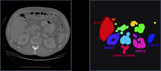
Kinds of Operation
- Seperate objects from background and from one another
- Aggregate pixels for each object
- Compute features for each object
Example: Red blood cell image
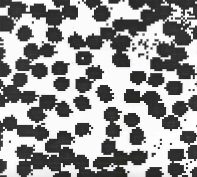
- Many blood cells are seperate objects
- Many touch - bad!
- Salt and pepper noise from thresholding
- How useable is this data
Results of analysis

- 63 separate objects detected
- Single cells have area about 50
- Noise spots
- Gobs of cells
Useful Operations
- Thesholding a gray-scale image
- Determine good threshold
- Connected components analysis
- All sorts of feature extractors, statistics (area, centroid, circularity, ...)
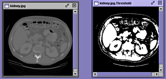
Thresholding

- Background is black
- Healthy cherry is bright
- Bruise is medium dark
- Histogram shows two cherry regions (black background has been removed)
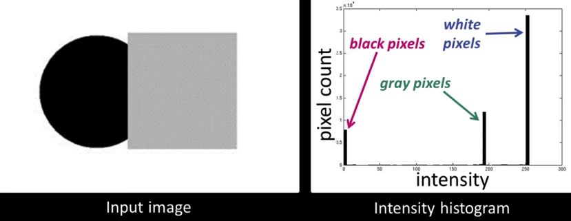
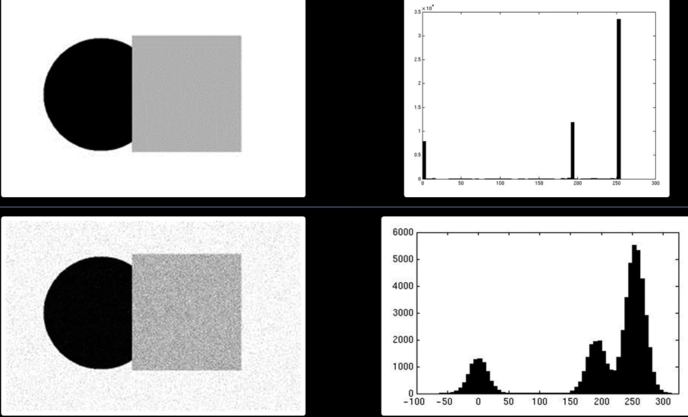
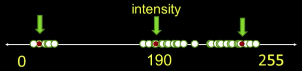
Histogram-Directed Thresholding
How can we use a histogram to separate an image into 2 (or several) different regions?

Automatic Thresholding: Otsu's Method
Assumption: The histogram is bimodal
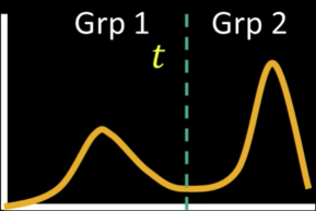
Method: Find the threshold $\color{blue}{t}$ that minimizes the weighted sum of within-group variances for the two groups that result from separating the gray tones at value $\color{blue}{t}$
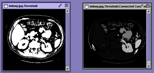
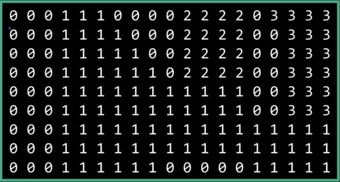
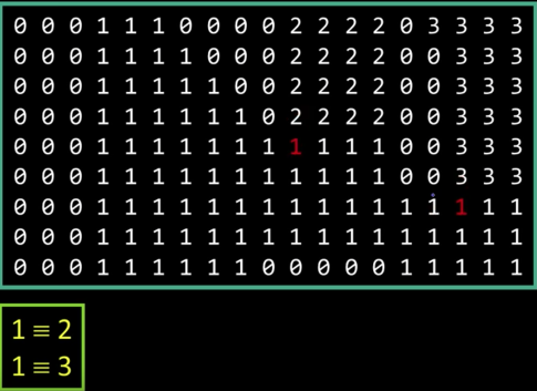
Connected Components
Methods
- Recursive Tracking (almost never used)
- Parallel Growing (needs parallel hardware)
- Row-by-Row (most common)
- Classical Algorithm
- Efficient Run-Length Algorithm (developed for speed in real industrial applications)
Algorithm
- CC = 0
- Scan across rows:
- IF 1 and connected:
- Propgate lowest label behind or above (4 or 8 connected). Remember conflicts
- If 1 and not connected:
- CC++ and label CC
- If 0:
- Label 0
- IF 1 and connected:
- Relabel based on table


Results
## from: https://stackoverflow.com/questions/46441893/connected-component-labeling-in-python
## it takes sometime
import cv2
import numpy as np

img = cv2.imread('imgs/eGaIy.jpg', 0)
img = cv2.threshold(img, 127, 255, cv2.THRESH_BINARY)[1]  # ensure binary
ret, labels = cv2.connectedComponents(img)

def imshow_components(labels):
    # Map component labels to hue val
    label_hue = np.uint8(179*labels/np.max(labels))
    blank_ch = 255*np.ones_like(label_hue)
    labeled_img = cv2.merge([label_hue, blank_ch, blank_ch])

    # cvt to BGR for display
    labeled_img = cv2.cvtColor(labeled_img, cv2.COLOR_HSV2BGR)

    # set bg label to black
    labeled_img[label_hue==0] = 0
    imshow(img)
    imshow(labeled_img)

imshow_components(labels)


Dilation and Erosion
Mathematical Morphology
Two basic operations
- Dilation
- Erosion
And several composite relations
- Closing and opeining
- Thinning and thickening ...
Dilation
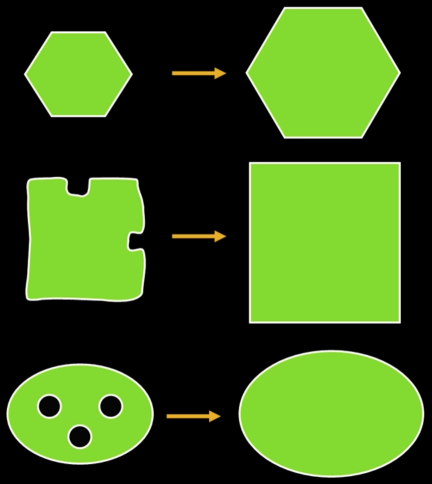
Dilation expands the connected sets of 1s of a binary image.
It can be used for:
- Growing features
- Filling holes and gaps
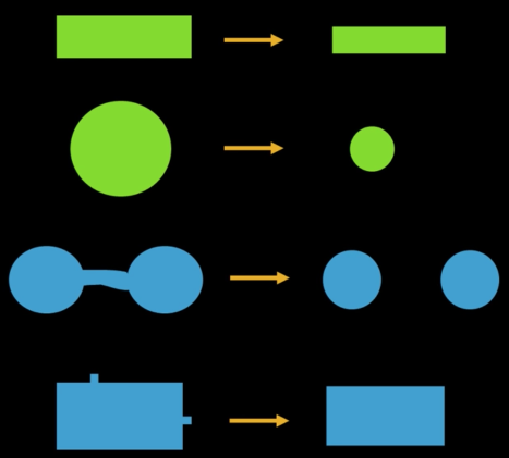
Errosion
Erosion shrinks the connected sets of 1s of a binary image.
It can be used for:
- Shrinking features
- Removing bridges, branches, protrusions
# Python program to demonstrate erosion and
# dilation of images.
import cv2
import numpy as np

# Reading the input image
jimg = imread('imgs/j.png')[:,:,0]

# Taking a matrix of size 5 as the kernel
kernel = np.ones((5,5), np.uint8)

img_erosion = cv2.erode(jimg, kernel, iterations=1)
img_dilation = cv2.dilate(jimg, kernel, iterations=1)

print("Original")
imshow(jimg)
print("Eroded")
imshow(img_erosion)
print("dilated")
imshow(img_dilation)


# dilation of images.
import cv2
import numpy as np

# Reading the input image
sadmessi = imread('imgs/sad_messi.jpg')[:,:,0]

# Taking a matrix of size 5 as the kernel
kernel = np.ones((5,5), np.uint8)

img_erosion = cv2.erode(sadmessi, kernel, iterations=1)
img_dilation = cv2.dilate(sadmessi, kernel, iterations=1)

print("Original")
imshow(sadmessi)
print("Eroded")
imshow(img_erosion)
print("dilated")
imshow(img_dilation)


Structuring Element
A shape mask used in basic morphological ops.
- Any shape, size that is digitally representable
- With a defined origin

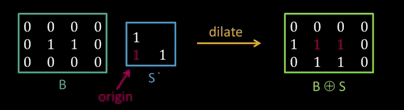
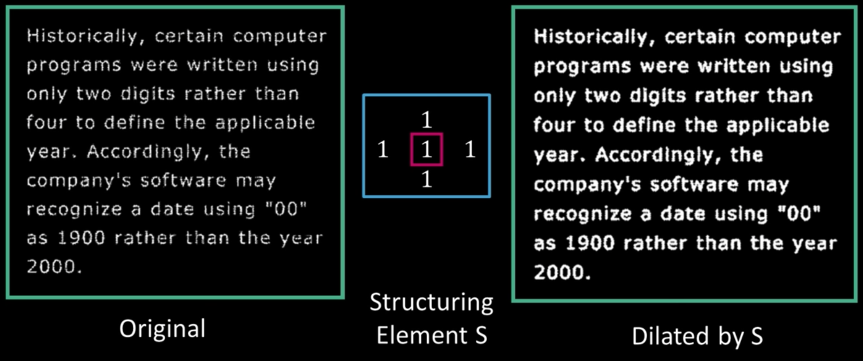
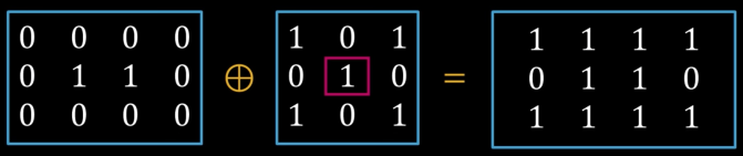
Dilation
Input: Binary image B, structuring element S
- Move S over B, placing origin at each pixel
- Considering only the 1-pixel location in S, compute the binary OR of corresponding elements in B
Binary text example
# Rectangular Kernel
print(cv2.getStructuringElement(cv2.MORPH_RECT,(5,5)))

# Elliptical Kernel
print(cv2.getStructuringElement(cv2.MORPH_ELLIPSE,(5,5)))

# Cross-shaped Kernel
print(cv2.getStructuringElement(cv2.MORPH_CROSS,(5,5)))
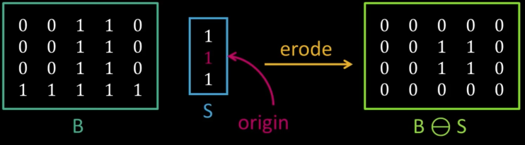
Erosion
Input: Binary image B, structuring element S
- Move S over B, placing origin at each pixel
- Considering only the 1-pixel location in S, compute the binary AND of corresponding elements in B
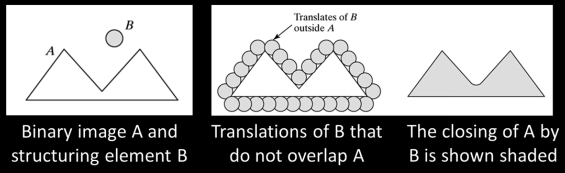
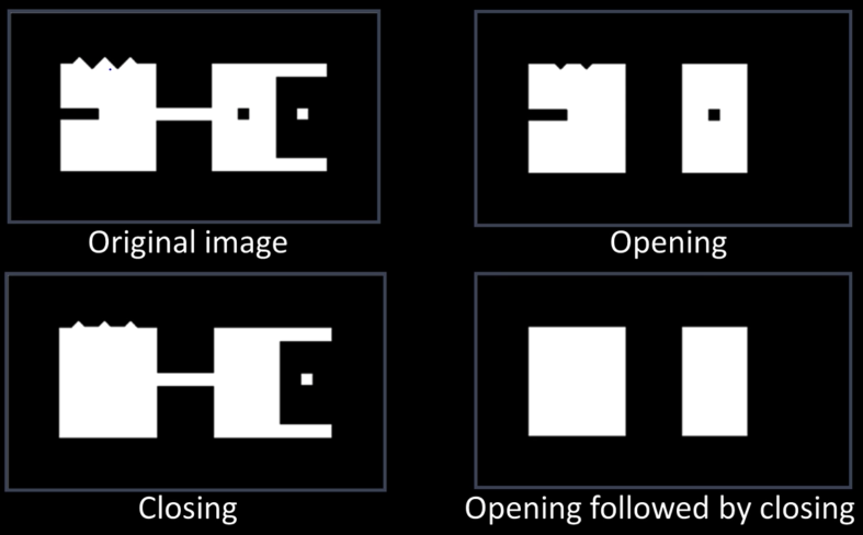
Opening
- Opening is the compund operation of erosion followed by dilation (with the same structuring element)
- Can show that opening of A by B is the union of all translations of B that fit entirely within A
- Opening is idempotent: Repeated operations has no further effects

Intuitively, the opening is the area we can paint when the brush has a footprint B and we are not allowed to paint outside A.
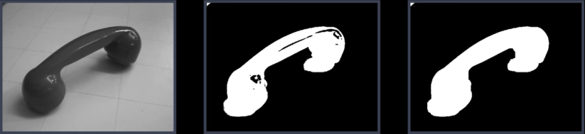
Opening example - cell colony
Use large structuring element that fits into big objects
- Structuring Element: 11 pixel disc

jblob = imread("imgs/j2.png")
opening = cv2.morphologyEx(jblob, cv2.MORPH_OPEN, kernel)
imshow(jblob)
imshow(opening)


kernel11 = np.ones((11,11), np.uint8)
messi_opening = cv2.morphologyEx(sadmessi, cv2.MORPH_OPEN, kernel)
imshow(sadmessi)
imshow(messi_opening)
messi_opening = cv2.morphologyEx(sadmessi, cv2.MORPH_OPEN, kernel11)
imshow(messi_opening)


Closing
- Closing is the compund operation dilation followed by erosion (with the same structuring element)
- Can show that closing of A by B is the complement of union of all translations of B that do not overlap with A
- Opening is idempotent: Repeated operations has no further effects
Intuitively, the closing is the area we can not paint when the brush has a footprint B and we are not allowed to paint inside A.
Closing Example - Segmentation
simple segmentation:
- Threshold
- Closing with disc of size 20
jblob2 = imread("imgs/j3.png")
closing = cv2.morphologyEx(jblob2, cv2.MORPH_CLOSE, kernel)
imshow(jblob2)
imshow(closing)


kernel11 = np.ones((11,11), np.uint8)
messi_closing = cv2.morphologyEx(sadmessi, cv2.MORPH_CLOSE, kernel)
imshow(sadmessi)
imshow(messi_closing)
messi_closing = cv2.morphologyEx(sadmessi, cv2.MORPH_CLOSE, kernel11)
imshow(messi_closing)


messi_opening = cv2.morphologyEx(sadmessi, cv2.MORPH_OPEN, kernel)
messi_closing = cv2.morphologyEx(messi_opening, cv2.MORPH_CLOSE, kernel)
imshow(sadmessi)
imshow(messi_closing)

Basic Morphological Algorithms
- Boundary extraction
- Region filling
- Extraction of connected components
- Convect Hull
- Thinning
- Skeletons
- Pruning
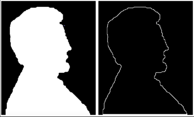
Boundry extraction
Let $\color{blue}{A \oplus B}$ denote the dilation of $\color{blue}{A}$ by $\color{blue}{B}$ and let $\color{blue}{A \ominus B}$ denote the erosion of $\color{blue}{A}$ by $\color{blue}{B}$
The boundary of $\color{blue}{A}$ can be computed as:
$$\color{blue}{A - (A \ominus B)}$$
where $\color{blue}{B}$ is a 3x3 square structuring element.
That is, we subtract from $\color{blue}{A}$ and erosion of it to obtain its boundary
Example of boundary extraction
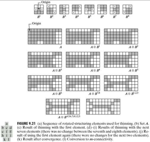
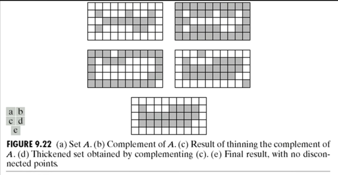
Thinning
$$\color{blue}{A \otimes B}$$ $$\color{blue}{= A - (A \oslash B)}$$ $$\color{blue}{= A \cap (A \oslash B)^C}$$
Thickening
$$\color{blue}{A \odot B = A \cup (A \oslash B)}$$
gradient = cv2.morphologyEx(jimg, cv2.MORPH_GRADIENT, kernel)
imshow(jimg)
imshow(gradient)

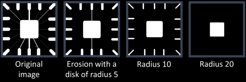
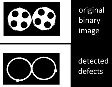
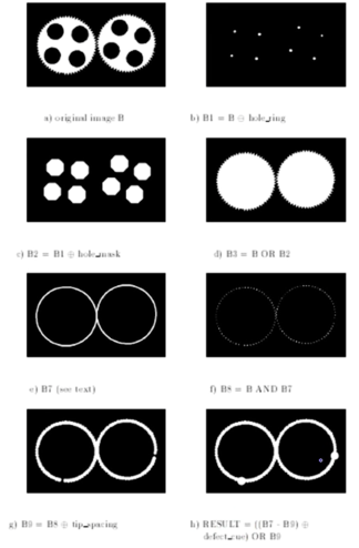
How Powerful is Morphology
It depends...
If almost "clean" binary images then very powerful to both clean up images and to detect variations from desired image.
- Example...
Geometric and Shape Properties
- area
- centroid
- perimeter
- perimeter length
- circularity
- elongation
- mean and standard deviation of radial distance
- bounding box
- extremal axis length from bounding box
- second order moments (row, column, mixed)
- lenghts and orientations of axes of best-fit ellipse
messi_gradient = cv2.morphologyEx(sadmessi, cv2.MORPH_GRADIENT, kernel)
imshow(sadmessi)
imshow(messi_gradient)

Amazing...
Messi...There are still more few battles. Get up and fight... You can't quit now... Fight until the last sweat.
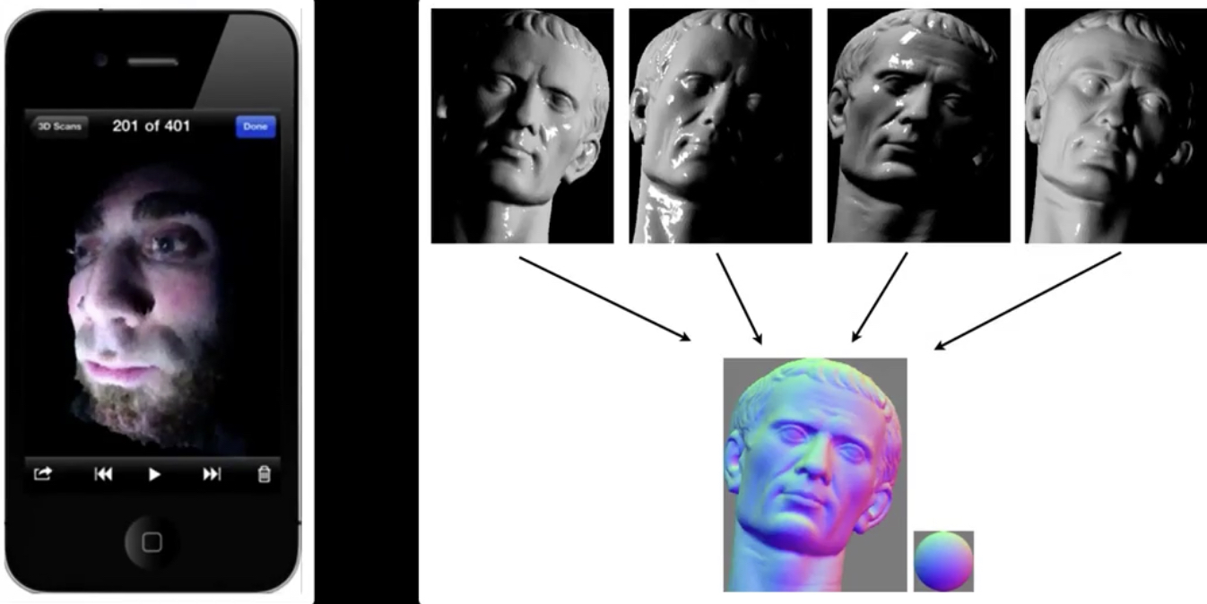
Motivation
- Determine shape
- What is the physical 3D structure of this object?
- Where does an object begin and the background begin?
- Find obstacles and map the environment
- How do I get my body/arm from A to B without hitting things?
- Others - tracking, dynamics, etc..
Weaknesses of images

Weaknesses of monocular vision


Potential solution: 3D sensing
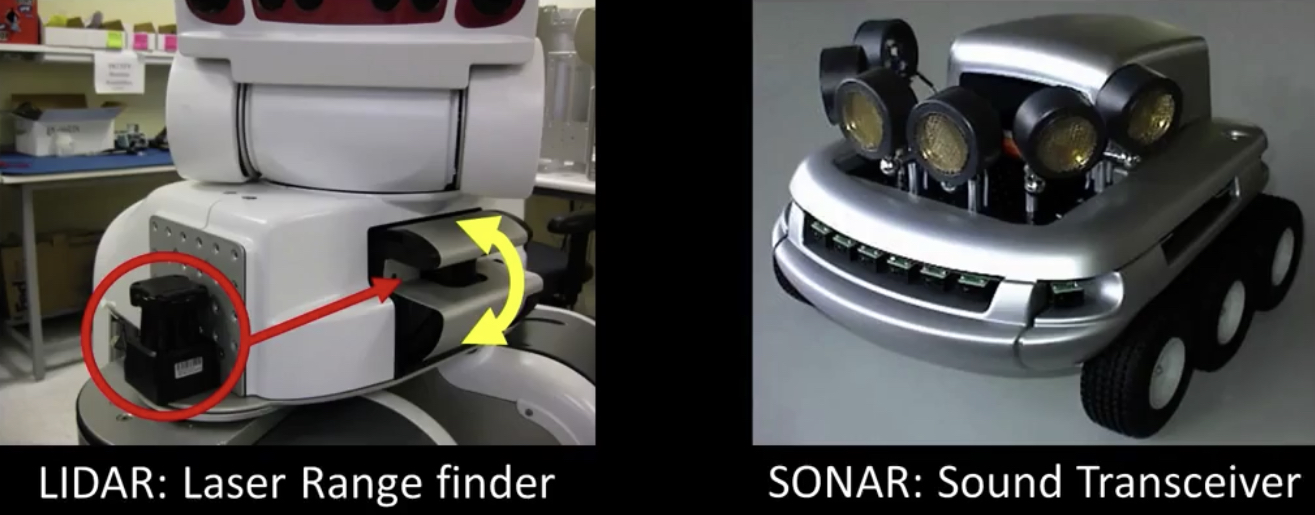
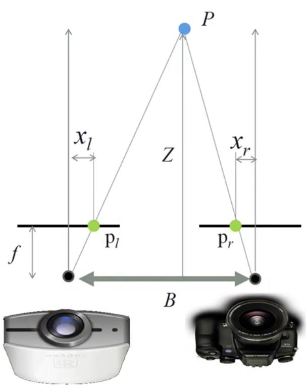
Passive 3D Sensing
Types of 3D sensing
- Passive 3D sensing
- Work with naturally occuring light
- Expoloit geometry or known properties of scenes
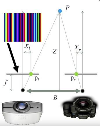
- Active 3D sensing
- Project light or sound out into the environment and see how it reacts
- Encode some pattern which can be found in the sensor
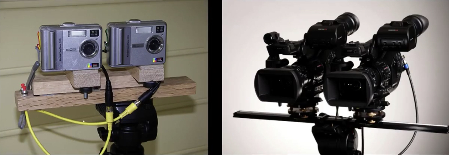
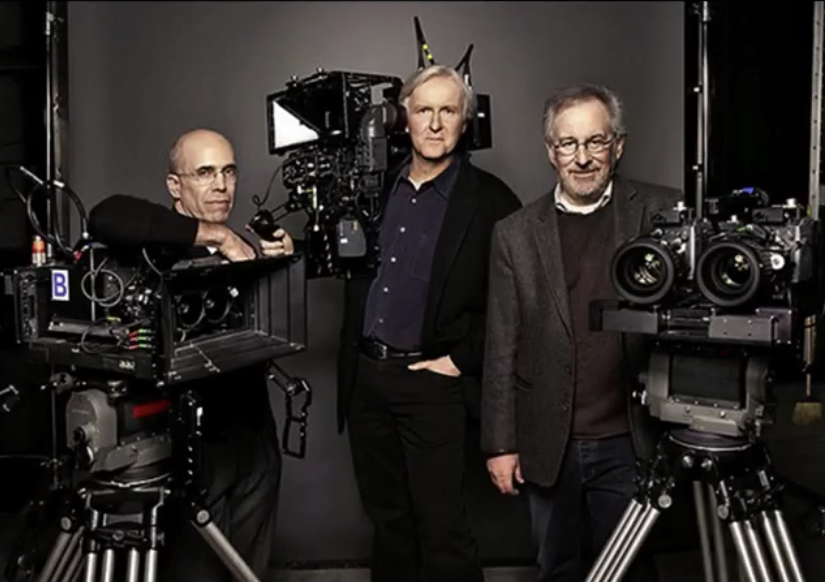
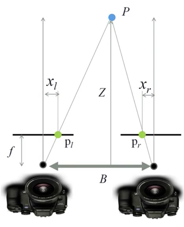
Passive: 3D sensors - stereo
Passive: 3D sensors - shape from (de)focus
Active 3D Sensing
Types of 3D sensing
Passive 3D sensing
- Work with naturally occuring light
- Expoloit geometry or known properties of scenes
Active 3D sensing
- Project light or sound out into the environment and see how it reacts
- Encode some pattern which can be found in the sensor
Active: Photometric stereo
Active: Time of flight
Bounce signal off of surface, record time to come back
$$\color{blue}{d = v * \frac{t}{2}}$$


Infrared and the Kinect

How does the Kinect work
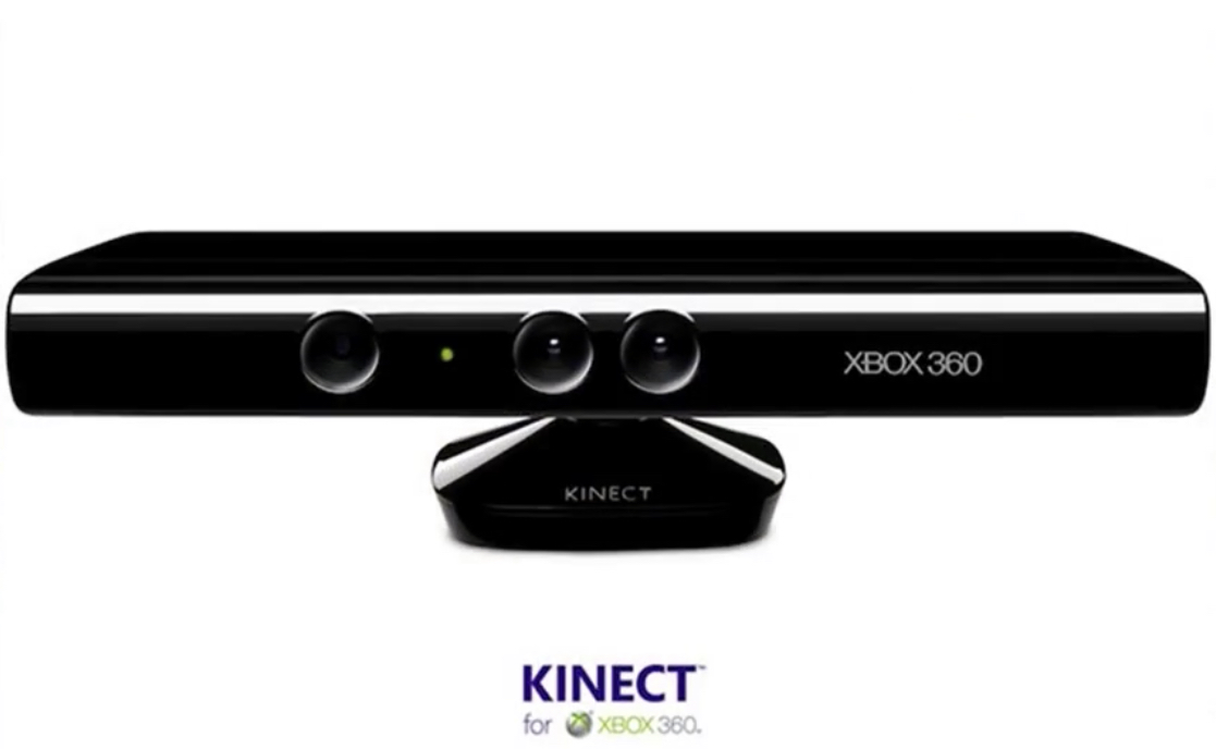
- Not public...
- But lots is known...
- The primesense patent(s) describes at least two ways...
How the Kinect sensor works - focus
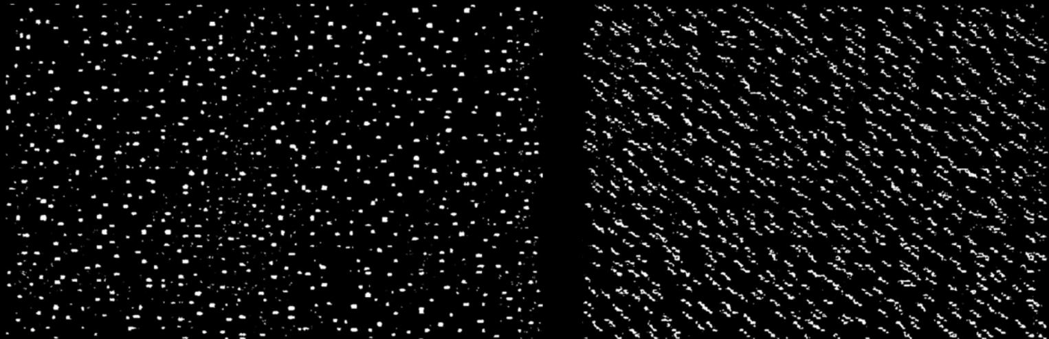
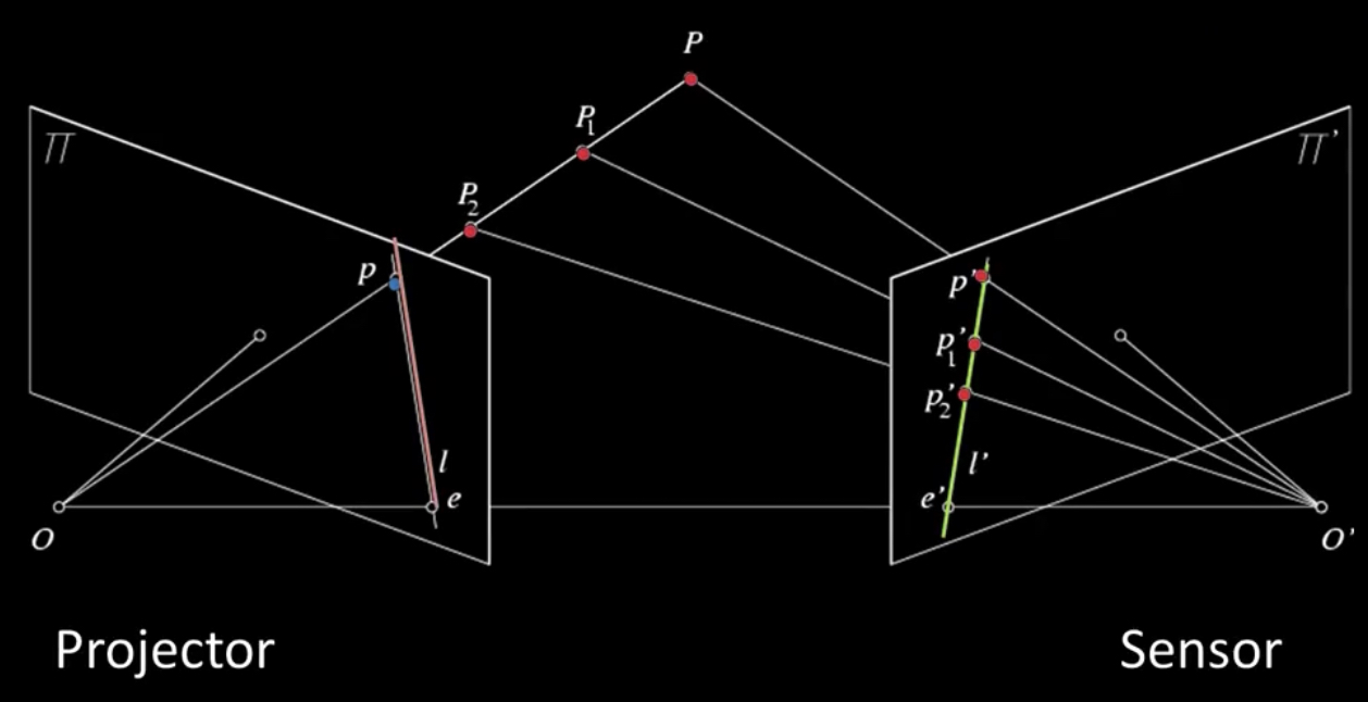
Cylindrical lens: Only focuses light in one direction
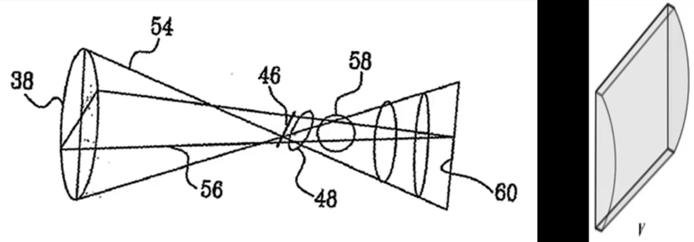
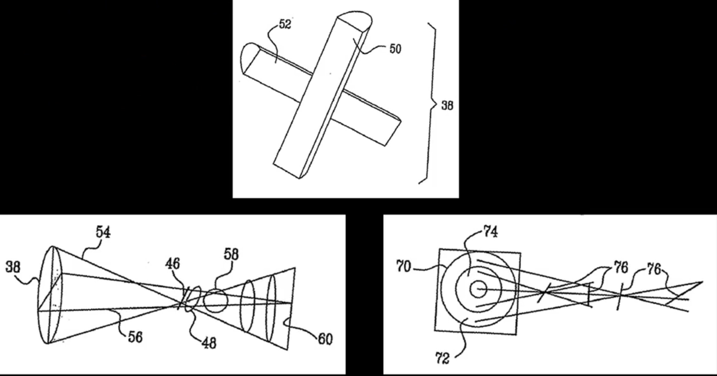
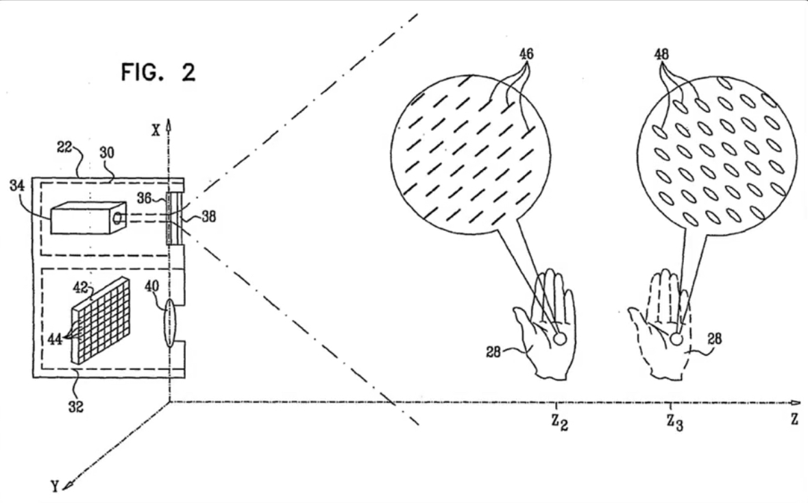
Orientation is a function of distance!
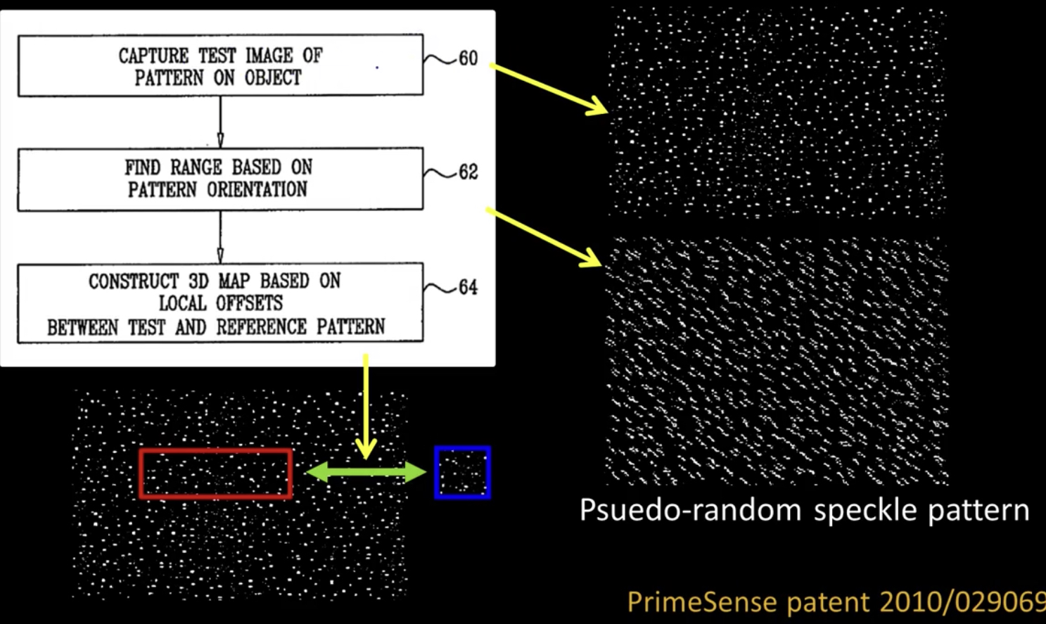

Algorithm
- Detect dots ("speckles") and label then unknown
Randomly select a region anchor, a dot with unknown depth
a. Windowed search via normalized cross correlation along scanline (check that best match score is greater than threshold; if not, mark as "invalid" and go to 2)
b. Region growing
- Neighboring pixels are added to a queue - For each pixel in queue, intialize by anchor's shift; then search small local neighborhood; if matched, add neighbors to queue - Stop when no pixels are left in the queue- Stop when all dots have known depths or are marked "invalid"
And Now a Video
Projected IR vs Natural Light Sterio
What are the advantages of IR?
- Works in low light conditions
- Does not rely on having textured objects
- Not confused by repeated scene textures
- can tailor algorithm to produce pattern
- Works outside, anywhere with sufficient light
- Resolution limited only by sensors, not projector
Difficulties with both
- Very dark surfaces may not reflect enough light
- Specular reflection in mirrors or mental causes trouble
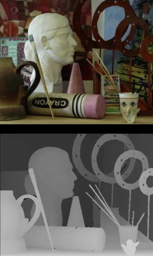
Depth Images
Representing depth scenes
Natural: depth image
A little more nuanced: point clouds
Depth images
Advantages
- Dense representation
- Gives intuition about occlusion and free space
- Depth discontinuities are just edges on the image
Disdvantages
- Viewpoint dependent, can't merge
- Doesn't capture physical geometry
- Need actual 3D location of camera(s)
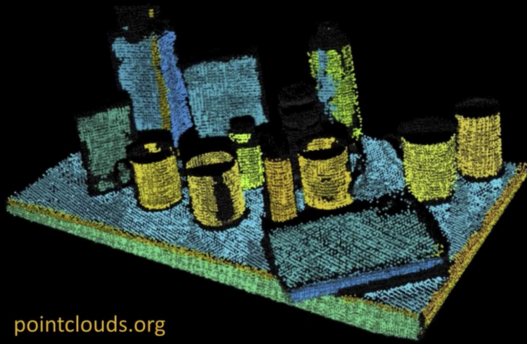
Point Clouds
Take every depth pixel and put it out in the world
- What can this representation tell us?
- What information do we lose?

Advantages
- Viewpoint independent
- Captures surface geometry
- Points represent physical locations
Disadvantages
- Sparse representation
- Lost information about free space and unknown space
- Variable density based on distance from sensor

- Biggest Advantage:
- PCL - Point Cloud Library

Point Feature Histogram and Software
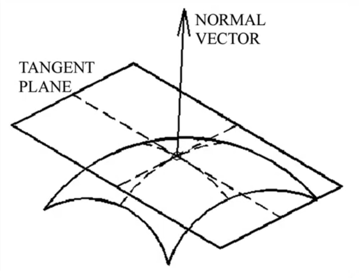
At a point, take a ball of points around it
For every pair of points, find the relationship between the two points and their normals
Must be frame independent

- Point Cloud Library (PCL)
- Robot Operating System (ROS)
- Framework for building systems
- http://www.ros.org
- Drivers for Kinet and other PrimeSense sensors
RANSAC Cylinder Segmentation