What does Recognition Involve
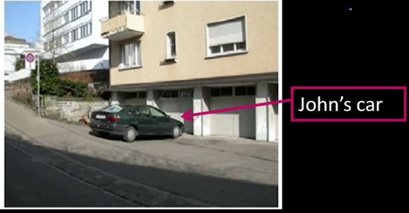
Verification

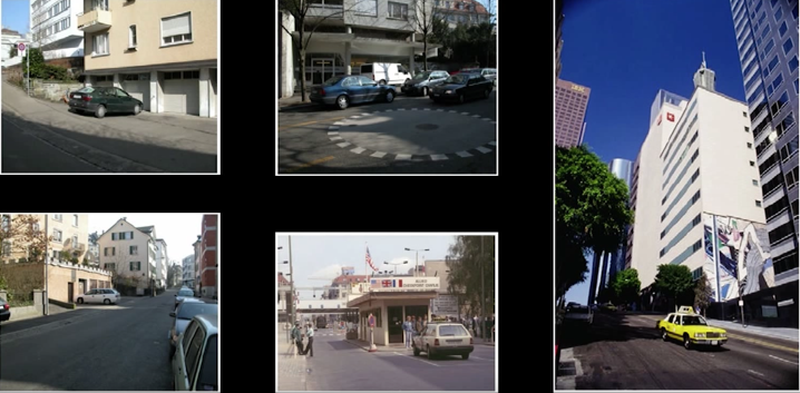
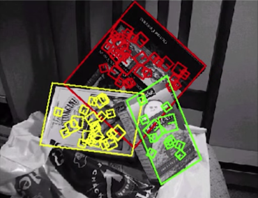
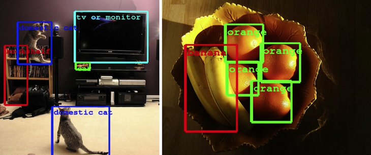
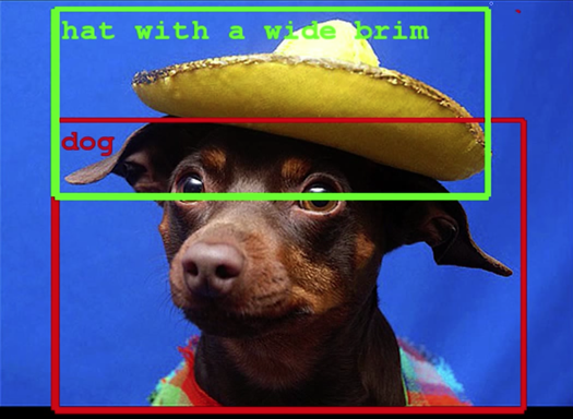
Detection
Identification
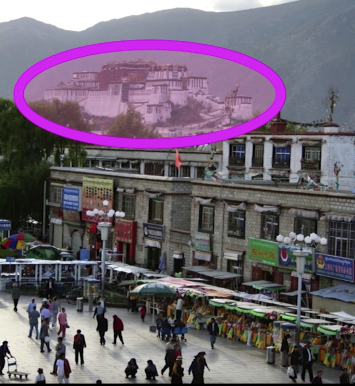
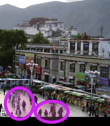
Object Categorization

Scene and context Categorization

Object Categorization
Instance-level recognition problem
Generic categorization problem
Object Categorization
Task: Given a (small) number of training images of a category, recognize a-priori unknown instances of that category and assign the correct category label
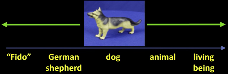
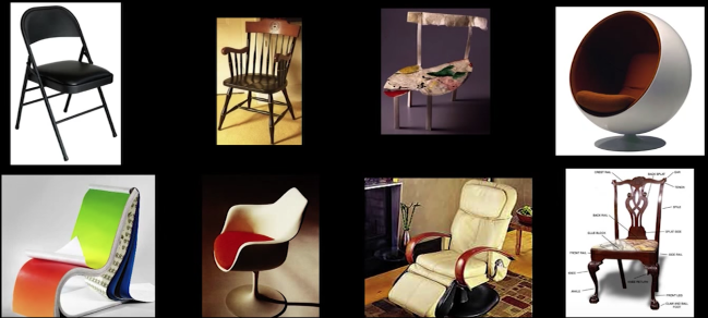
Visual Object Categories
Basic Level Categories in human categorization [Rosch 76, Lakoff 87]
- The highest level at which category members have similar perceived shape
- The highest level at which a single mental image reflects the entire category
- The level at which human subjects are usually fastest at identifying category members
- The first level named and understood by children
- The highest level at which a person uses similar motor actions for interaction with category members

Other Types of Categories
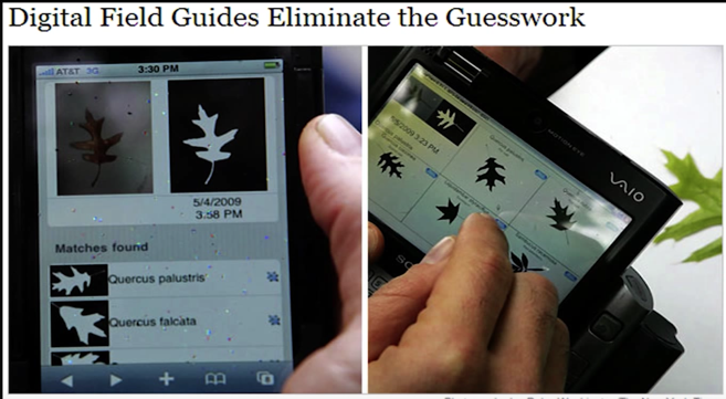
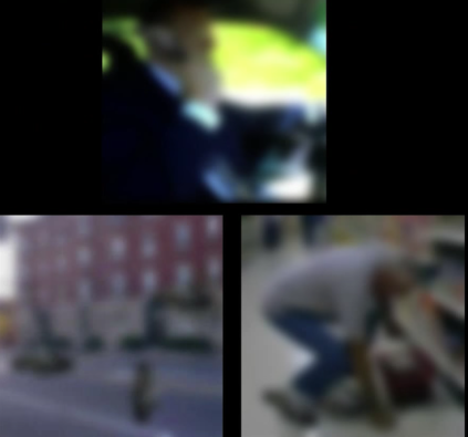
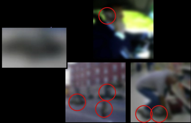
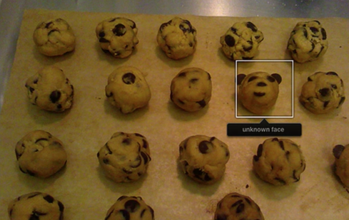
Using Recognition

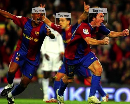
I swear I didn't cheat, this the image in the lecture

Challenges

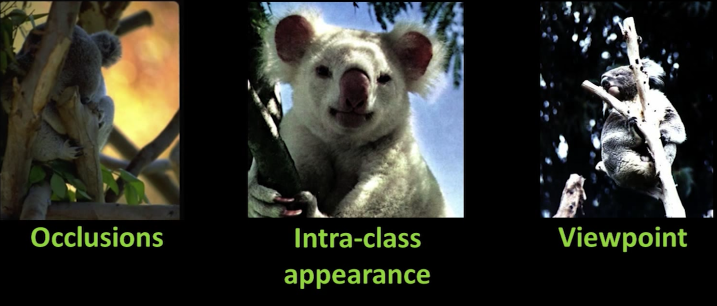
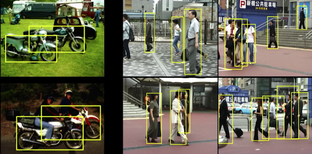
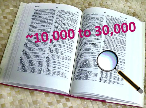
Complexity
- Thousands to millions of pixels in an image
- 3,000-30,000 human recognizable object categories
- 30+ degrees of feedom in the pose of articulated objects (humans)
- Billions of images indexed by Google Image Search
- In 2011, 6 billion photos uploaded per month
- Approximately one billion camera phones sold in 2013
- About half of the cerebral cortex in primates is devoted to processing visual information [Felleman and van Essen 1991]
What Works?
What worked most reliably "yesterday"

Going forward
- These days much of strong label "recognition" is really machine learning applied to patterns of pixel intensities.
- To cover this would require deep understanding of machine learning. Another class - or six...
- We'll focus on some general principals of generative vs discriminative methods and the representations of the image that they use
- To cover this would require deep understanding of machine learning. Another class - or six...
- And then we'll spend some time on activity recognition from video
Supervised Classification
Given a collection of labeled examples, come up with a function that will predict the labels of new examples.
How good is the function we come up with to do the classification? (What does "good" mean?)
Depends on:
- What mistakes does it make
- Cost associated with the mistakes
Since we know the desired labels of training data, we want to minimize the expected misclassification
Two general strategies
Use the training data to build representative probability model; separately model class-conditional densities and priors (Generative)
Directly construct a good decision boundary, model the posterior (Discriminative)
Generative
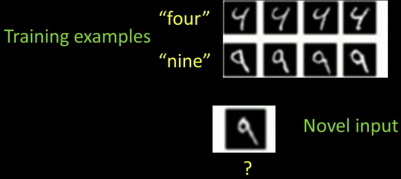
Given Labeled training examples, predict labels for new examples
- Notation: ($4\rightarrow 9$) - object is a '4' but you call it a '9'
- We'll assume the cost of ($X\rightarrow X$) is zero
Consider the two-class (binary) decision problem:
- L($4\rightarrow 9$): Loss of classifying a 4 as a 9
- L($9\rightarrow 4$): Loss of classifying a 9 as a 4
Risk of a classifier startegy $S$ is expected loss:
$$R(S) = Pr(4\rightarrow 9|\text{using S}) L(4\rightarrow 9) + Pr(9\rightarrow 4|\text{using S}) L(9\rightarrow 4)$$
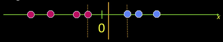
Minimal Risk
Supervised classification: minimal risk

If we choose class "four" at boundary, expected loss is:
$$ = P(\text{class is }9|x)L(9\rightarrow 4) + P(\text{class is }4|x)L(4\rightarrow 4)$$ $$ = P(\text{class is }9|x)L(9\rightarrow 4)$$
If we choose class "nine" at boundary, expected loss is: $$ = P(\text{class is }4|x)L(4\rightarrow 9)$$
So, best decision boundary is at point $x$ where:
$$P(\text{class is }9|x)L(9\rightarrow 4) = P(\text{class is }4|x)L(4\rightarrow 9)$$
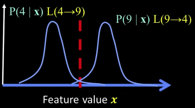
How to evaluate $P(\text{class is }9|x)$ and $P(\text{class is }4|x)$?
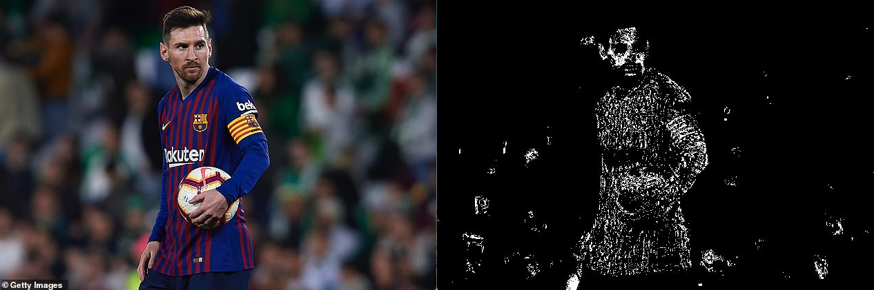
Example Learning Skin Colors
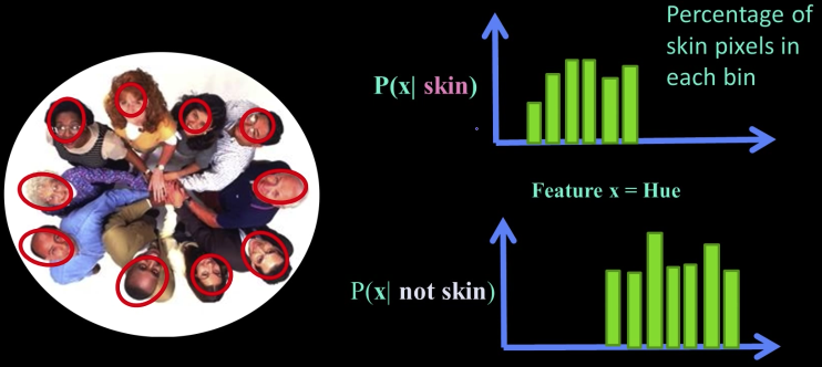
$$P(skin|x) = \frac{P(x|skin)P(skin)}{P(x)}$$
$P(skin|x)$: posterior
$P(x)$: prior
$P(x|skin)$: likelihood (we have this from the data)
$$P(skin|x) \propto P(x|skin)P(skin)$$
Where does the prior come from?
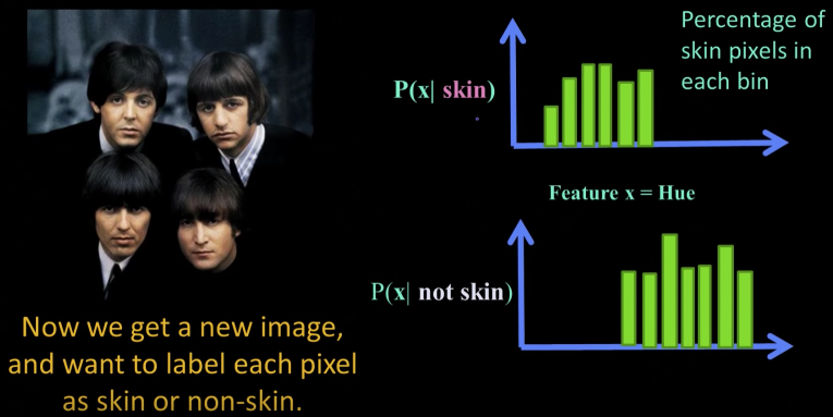
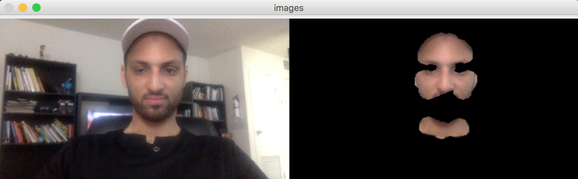
Skin detection using OpenCV
https://www.pyimagesearch.com/2014/08/18/skin-detection-step-step-example-using-python-opencv/
# """
# Run the following code in the terminal so you can exit gracefully.
# Source: https://www.pyimagesearch.com/2014/08/18/skin-detection-step-step-example-using-python-opencv/
# """
import numpy as np
import argparse
import cv2
def resize(image, width=None, height=None, inter=cv2.INTER_AREA):
# initialize the dimensions of the image to be resized and
# grab the image size
dim = None
(h, w) = image.shape[:2]
# if both the width and height are None, then return the
# original image
if width is None and height is None:
return image
# check to see if the width is None
if width is None:
# calculate the ratio of the height and construct the
# dimensions
r = height / float(h)
dim = (int(w * r), height)
# otherwise, the height is None
else:
# calculate the ratio of the width and construct the
# dimensions
r = width / float(w)
dim = (width, int(h * r))
# resize the image
resized = cv2.resize(image, dim, interpolation=inter)
# return the resized image
return resized
# define the upper and lower boundaries of the HSV pixel
# intensities to be considered 'skin'
lower = np.array([0, 48, 80], dtype = "uint8")
upper = np.array([20, 255, 255], dtype = "uint8")
camera = cv2.VideoCapture(0)
# keep looping over the frames in the video
while True:
# grab the current frame
(grabbed, frame) = camera.read()
# resize the frame, convert it to the HSV color space,
# and determine the HSV pixel intensities that fall into
# the speicifed upper and lower boundaries
frame = resize(frame, width = 400)
converted = cv2.cvtColor(frame, cv2.COLOR_BGR2HSV)
skinMask = cv2.inRange(converted, lower, upper)
# apply a series of erosions and dilations to the mask
# using an elliptical kernel
kernel = cv2.getStructuringElement(cv2.MORPH_ELLIPSE, (11, 11))
skinMask = cv2.erode(skinMask, kernel, iterations = 2)
skinMask = cv2.dilate(skinMask, kernel, iterations = 2)
# blur the mask to help remove noise, then apply the
# mask to the frame
skinMask = cv2.GaussianBlur(skinMask, (3, 3), 0)
skin = cv2.bitwise_and(frame, frame, mask = skinMask)
# show the skin in the image along with the mask
cv2.imshow("images", np.hstack([frame, skin]))
# if the 'q' key is pressed, stop the loop
if cv2.waitKey(1) & 0xFF == ord("q"):
break
camera.release()
cv2.destroyAllWindows()
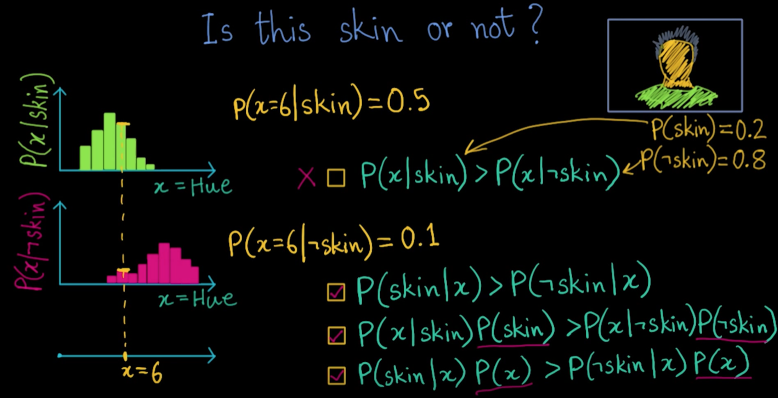
Bayes rule in (ab)use
Likelihood ration test (assuming cost of errors is the same):
If $P(x|skin)P(skin) > P(x|\sim skin)P(\sim skin)$ classify $x$ as skin (Bayes rule)
(if the costs are different just re-weight)
...but I don't really know prior $P(skin)$...
...but I can assume it it some constant $\Omega$...
... so with some training data I can estimate $\Omega$...
... and with the same training data I can measure the likelihood densities of both $P(x|skin)$ and $P(x|\sim skin)$...
So... I can more or less come up with a rule...
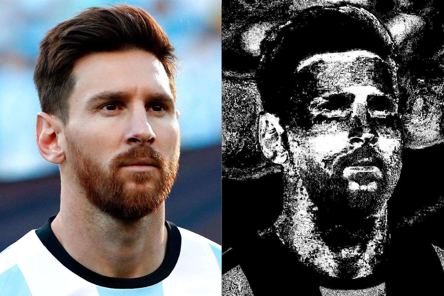
Now for every pixel in a new image, we can estimate probability that it is generated by skin:
If $P(skin|x) > \theta$ classify as skin; otherwise not
# Example of Naive Bayes implemented from Scratch in Python
## Source: https://machinelearningmastery.com/naive-bayes-classifier-scratch-python/
"""
The test problem we will use in this tutorial is the Pima Indians Diabetes problem.
This problem is comprised of 768 observations of medical details for Pima indians patents. The records describe instantaneous measurements taken from the patient such as their age, the number of times pregnant and blood workup. All patients are women aged 21 or older. All attributes are numeric, and their units vary from attribute to attribute.
Each record has a class value that indicates whether the patient suffered an onset of diabetes within 5 years of when the measurements were taken (1) or not (0).
This is a standard dataset that has been studied a lot in machine learning literature. A good prediction accuracy is 70%-76%.
Below is a sample from the pima-indians.data.csv file to get a sense of the data we will be working with (update: download from here).
"""
import csv
import random
import math
def loadCsv(filename):
lines = csv.reader(open(filename, "r"))
dataset = [l for l in lines]
for i in range(len(dataset)):
dataset[i] = [float(x) for x in dataset[i]]
return dataset
def splitDataset(dataset, splitRatio):
trainSize = int(len(dataset) * splitRatio)
trainSet = []
copy = list(dataset)
while len(trainSet) < trainSize:
index = random.randrange(len(copy))
trainSet.append(copy.pop(index))
return [trainSet, copy]
def separateByClass(dataset):
separated = {}
for i in range(len(dataset)):
vector = dataset[i]
if (vector[-1] not in separated):
separated[vector[-1]] = []
separated[vector[-1]].append(vector)
return separated
def mean(numbers):
return sum(numbers)/float(len(numbers))
def stdev(numbers):
avg = mean(numbers)
variance = sum([pow(x-avg,2) for x in numbers])/float(len(numbers)-1)
return math.sqrt(variance)
def summarize(dataset):
summaries = [(mean(attribute), stdev(attribute)) for attribute in zip(*dataset)]
del summaries[-1]
return summaries
def summarizeByClass(dataset):
separated = separateByClass(dataset)
summaries = {}
for classValue, instances in separated.items():
summaries[classValue] = summarize(instances)
return summaries
def calculateProbability(x, mean, stdev):
exponent = math.exp(-(math.pow(x-mean,2)/(2*math.pow(stdev,2))))
return (1 / (math.sqrt(2*math.pi) * stdev)) * exponent
def calculateClassProbabilities(summaries, inputVector):
probabilities = {}
for classValue, classSummaries in summaries.items():
probabilities[classValue] = 1
for i in range(len(classSummaries)):
mean, stdev = classSummaries[i]
x = inputVector[i]
probabilities[classValue] *= calculateProbability(x, mean, stdev)
return probabilities
def predict(summaries, inputVector):
probabilities = calculateClassProbabilities(summaries, inputVector)
bestLabel, bestProb = None, -1
for classValue, probability in probabilities.items():
if bestLabel is None or probability > bestProb:
bestProb = probability
bestLabel = classValue
return bestLabel
def getPredictions(summaries, testSet):
predictions = []
for i in range(len(testSet)):
result = predict(summaries, testSet[i])
predictions.append(result)
return predictions
def getAccuracy(testSet, predictions):
correct = 0
for i in range(len(testSet)):
if testSet[i][-1] == predictions[i]:
correct += 1
return (correct/float(len(testSet))) * 100.0
def main():
filename = 'nvb_data.csv'
splitRatio = 0.67
dataset = loadCsv(filename)
trainingSet, testSet = splitDataset(dataset, splitRatio)
print('Split %d rows into train=%d and test=%d rows' % (len(dataset), len(trainingSet), len(testSet)))
# prepare model
summaries = summarizeByClass(trainingSet)
# test model
predictions = getPredictions(summaries, testSet)
accuracy = getAccuracy(testSet, predictions)
print('Accuracy: %f' % accuracy)
main()
For example on Naive Bayes on images https://github.com/Chinmoy007/Skin-detection
More General Generative Models
For a given measurement $x$ and set of classes $c_i$ choose $c*$ by:
$$c* = argmax_c P(c|x) = argmax_c P(c)P(x|c)$$
Continuous generative models
- If $x$ is continuous, need likelihood density model of $p(x|c)$
- Typically parametric - Gaussian or mixture of Gaussians
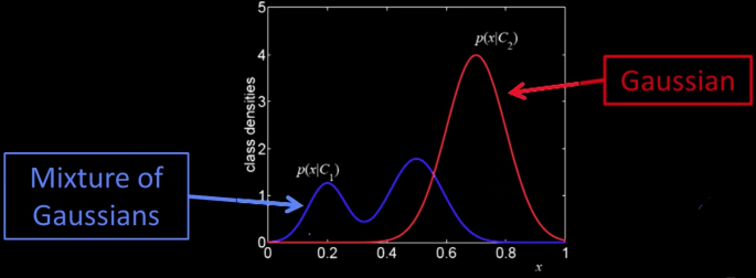
- Why not just some histogram or some KNN (Parzen window) method?
- You might...
- But you would need lots and lots of data everywhere you might get a point
- The whole point of modeling with a parameterized model is not to need lots of data
Summary of Generative Models
- Firm probabilistic grounding
- Allows inclusing of prior knowledge
- Parametric modeling of likelihood permits using small number of examples
- New classes do not perturb previous models
- Others:
- Can take advantage of unlabelled data
- Can be used to generate samples
Downsides
- And just where did you get those priors?
- Why are you modeling those obviously non-C points?
- The example hard cases aren't special
- If you have lots of data, doesn't help
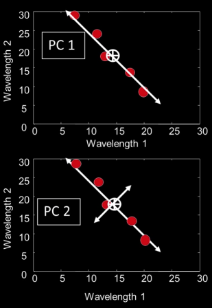
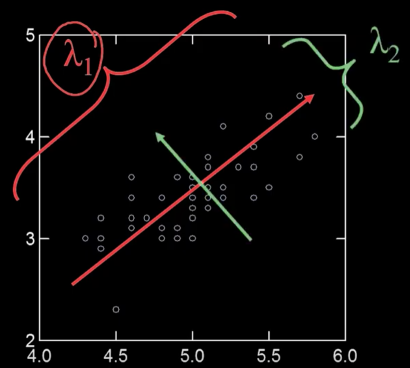
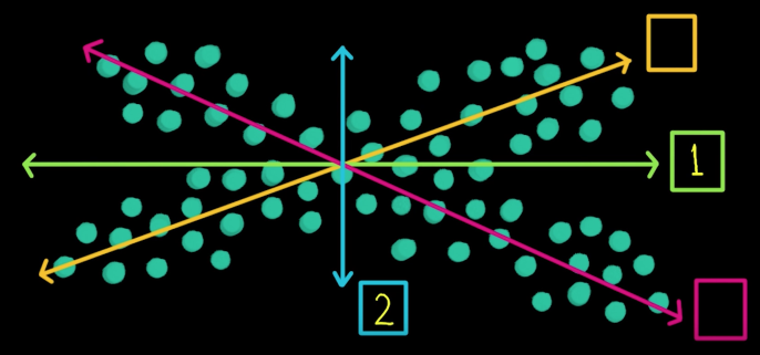
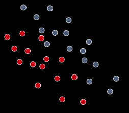
Principle Components
- Principle components are all about the directions in a feature space along which points have the greatest variance
First PC is the direction of maximum variance. Technically (and mathematically) it's from the origin, but we actually mean the mean
Subsequent PCs are orthogonal to previous PCs and describe maximum residual variance
2D Example Fitting a line
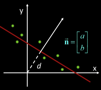
$$E(a,b,d) = \sum_i (ax_i+by_i-d)^2$$
$$E = \sum_i [a(x_i-\overline{x}) + b(y_i-\overline{y})]^2 = ||Bn||^2$$
where $B = \begin{bmatrix} x_1-\overline{x} & y_1-\overline{y}\\ x_2-\overline{x} & y_2-\overline{y}\\ ... & ...\\ x_n-\overline{x} & y_n-\overline{y}\\ \end{bmatrix}$
So minimize $||Bn||^2$ subject to $||n||=1$ gives axis of least inertia
Algebraic Interpretation
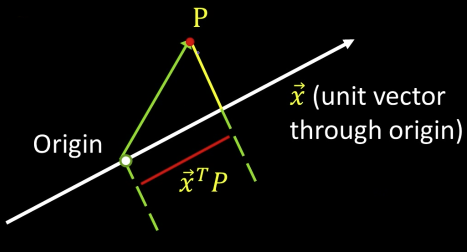
Minimizing sum of squares of distances to the line is the same as *maximizing the sum of squares of the projections on that line*
Trick: How is the sum of squares of projection lengths expressed in algebraic terms

Our goal: max($x^TB^TBx)$, subject tp $x^Tx=1$
maximize $E=x^TMx$ subject to $x^Tx$=1 ($M=B^TB$)
$$E' = x^TMx + \lambda(1-x^Tx)$$
$$\frac{\partial E'}{\partial x} = 2Mx + 2\lambda x$$
$$\frac{\partial E'}{\partial x} = - \rightarrow MX = \lambda x \,\,\,\, \text{(x is an eigenvector of}\,\,B^TB)$$
Yet another algebraic interpretation
$$B^TB = \begin{bmatrix} \sum_{i=1}^n x^2_i& \sum_{i=1}^n x_iy_i\\ \sum_{i=1}^n x_iy_i& \sum_{i=1}^n y^2_i \end{bmatrix}\,\,\,\text{if about origin}$$
So the principal components are the orthogonal directions of the covariance matrix of a set points
$$\color{blue}{B^TB = \sum xx^t\,\,\,\text{if about origin}}$$
$$\color{blue}{B^TB = \sum (x-\overline{x})(x-\overline{x})^T\,\,\,\text{otherwise-outer product}}$$
</font>
So the principal components are the orthogonal directions of the *covariance matrix of a set points
Eigenvectors
How many eigenvectors are there?
- For real symmetric matrices of size NxN
- Except in degenerate cases when eigenvalues repeat, there are N distinct eigenvectors
"""
===============
Demo PCA
Source: source: https://www.science-emergence.com/Articles/Analyse-en-composantes-principales-avec-python/
===============
"""
from sklearn.decomposition import PCA
import numpy as np
import matplotlib.pyplot as plt
mean = [0,0]
cov = [[40,35],[35,40]]
x1,x2 = np.random.multivariate_normal(mean,cov,1000).T
X = np.c_[x1,x2]
plt.xlim(-25.0,25.0)
plt.ylim(-25.0,25.0)
plt.grid()
plt.scatter(X[:,0],X[:,1])
pca = PCA(n_components=2)
pca.fit(X)
print(pca.explained_variance_ratio_)
print(pca.components_)
axis = pca.components_.T
axis /= axis.std()
x_axis, y_axis = axis
plt.plot(0.1 * x_axis, 0.1 * y_axis, linewidth=1 )
plt.quiver(0, 0, x_axis, y_axis, zorder=11, width=0.01, scale=6, color='red')

Dimensionality Reduction
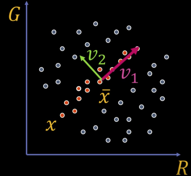
We can represent the orange points with only their $v_1$ coordinates
Higher Dimensions
- Suppose each data point is N-dimensional
$$var(v) = \sum_x||(x-\overline{x})^T\cdot v||$$ $$ = v^TAv\,\,\text{where}\,\, A = \sum(x-\overline{x})(x-\overline{x})$$
$(x-\overline{x})(x-\overline{x})$: outer product
- The eigen vector largest with the largest eigenvalue $\lambda$ captures the most variation among training vector $x$
"""
===============
Demo PCA in 2D
Source: https://scipy-lectures.org/packages/scikit-learn/auto_examples/plot_pca.html
===============
"""
############################################################
# Load the iris data
from sklearn import datasets
iris = datasets.load_iris()
X = iris.data
y = iris.target
############################################################
# Fit a PCA
from sklearn.decomposition import PCA
pca = PCA(n_components=2, whiten=True)
pca.fit(X)
############################################################
# Project the data in 2D
X_pca = pca.transform(X)
############################################################
# Visualize the data
target_ids = range(len(iris.target_names))
from matplotlib import pyplot as plt
fig ,ax = plt.subplots(nrows=2)
fig.set_size_inches((6, 5))
ax[0].scatter(X_pca[:, 0], X_pca[:, 1])
for i, c, label in zip(target_ids, 'rgbcmykw', iris.target_names):
ax[1].scatter(X_pca[y == i, 0], X_pca[y == i, 1],
c=c, label=label)
plt.legend()

The Space of All Face Images
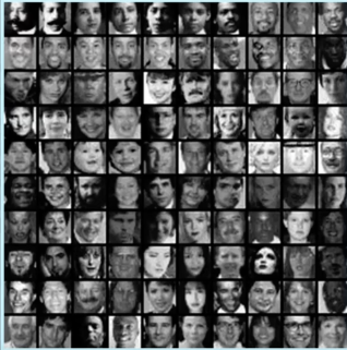
When viewed as vectors of pixel values, face images are extremely high-dimensional
- 100x100 image = 10,000 dimensions
However, relatively few 10,000-dimensional vectors correspond to valid face images
- We want to effectively model subspace of face images
We want to construct a low-dimensional linear subspace that best explains the variation in the set of face images
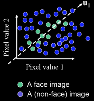
Principal Component Analysis
- Given: $\color{blue}{M}$ data points $\color{blue}{x_1,...x_M}\text{ in }\color{blue}{R^d}\,\text{where}\,\color{blue}{d}$ is big
- We want some direcions in $\color{blue}{R^d}$ that capture most of the variation of the $\color{blue}{x_i}$. The coefficients would be: $$\color{blue}{u(x_i) = u^T(x_i-\mu)}$$
($\color{blue}{\mu}$: mean of data points)
What unit vector $\color{blue}{u}$ in $\color{blue}{R^d}$ captures the most variance of the data?
Direction that maximizes the variance of the projected data:
$$var(u) = \frac{1}{M}\sum_{i=1}^Mu^T (x_i - \mu)(u^T(x_i - \mu))^T$$
Where: $u^T (x_i - \mu)$: Projection of data point
$$ = u^T\left [\frac{1}{M}\sum_{i=1}^N(x_i - \mu)(x_i-\mu)^T\right ]u$$
Where: $\frac{1}{M}\sum_{i=1}^N(x_i - \mu)(x_i-\mu)^T$: Covariance matrix of data
$$ = \color{blue}{u^T}\color{green}{\sum}\color{blue}{u}$$
Since $\color{blue}{u}$ is a unit vector that can be expressed in terms of some linear sum of the eigenvectors of $\color{blue}{\sum}$, then direction of $\color{blue}{u}$ that maximizes the variance is the eigenvector associated with the largest eigenvalue of $\color{blue}{\sum}$
- The direction that captures the maximum covariance of the data is the eigenvector corresponding to the largest eigenvalue of the data covariance matrix
- Furthermore, the top k orthogonal directions that capture the most variance of the data are the k eigenvectors corresponding to the k largest eigenvalues
- But first, we'll need the PCA d>>>n trick...
The Dimensionality Trick
Let $\color{blue}{\Phi_i}$ be the (very big vector length d) that is face image I with the mean image subtracted.
Define: $$\color{blue}{C = \frac{1}{M}\sum \Phi_i \Phi_i^T = AA^T}$$
where $\color{blue}{A =\Phi_1 \Phi_2 ... \Phi_M}$ is the matrix of faces, and is $\color{blue}{d\times M}$
Note: C is a huge $d\times d$ matrix (remember d is the length of the vector of the image).
So $C = AA^T$ is a huge matrix.
But consiter $\color{blue}{A^TA}$. It is only $M\times M$. Finding those eigenvalues is easy
Suppose $\color{blue}{v_i}$ is an eigenvector $\color{blue}{A^TA}$: $$\color{blue}{A^TAv_i = \lambda v_i}$$
Premultiply by $\color{blue}{A}$:
$$\color{blue}{AA^T}\color{green}{Av_i} = \color{blue}{\lambda}\color{green}{Av_i}$$
So: $\color{green}{Av_i}$ are the eigenvectors of $\color{blue}{C = AA^T}$
How Many Eigenvectors Are There
- If I had $M > d$ then there would be $d$. But $M << d$
- So intuition would say there are $M$ of them
- But wait: if 2 points in 3D, how many eigenvectors? 3 points?
- Subtracting out the mean yields $M-1$
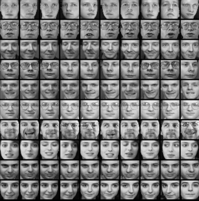
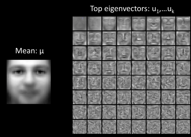
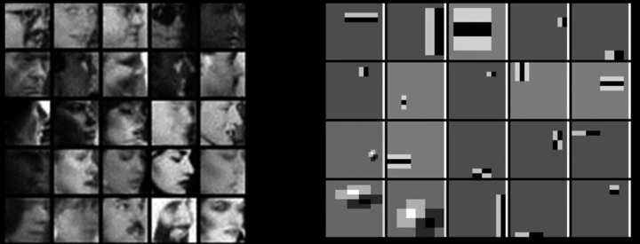
Eigenfaces
Eigenfaces: Key idea (Truk and pentland, 1991)
- Assume that most face images lie on a low-dimensional subspace determined by the first k ($\color{blue}{k<<<d}$) directions of maximum variance
- Use PCA to determine the vectors or "eigenfaces" $u_1,u_2,...u_k$ that span that subspace
- Represent all face images in the dataset as linear combinations of eigenfaces. Find the coefficients by dot product.
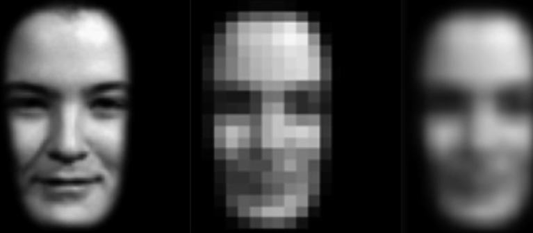
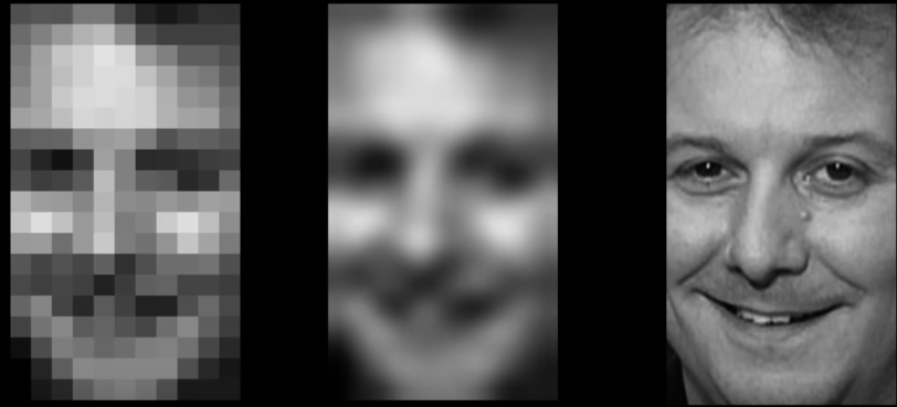
Eigenfaces example
Eigenfaces example
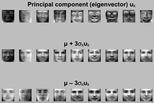
- Face X in "face space" coordinates (dot products):

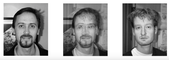
Recognition with Eigenfaces
Given novel image $\color{blue}{x}$:
- Project onto subspace:
$$[w_1,...,w_k] = [u^T_1(x-\mu),...,u^T_k(x-\mu)]$$
- Optional: check reconstruction error $x-\hat{x}$ to determine whethere image is really a face
- Classify as closest training face in k-dimentional subspace
- This is why it's a generative model
"""
===============
Demo Eigenfaces
Source: https://pythonmachinelearning.pro/face-recognition-with-eigenfaces/
===============
"""
import matplotlib.pyplot as plt
from sklearn.model_selection import train_test_split
from sklearn.datasets import fetch_lfw_people
from sklearn.metrics import classification_report
from sklearn.decomposition import PCA
from sklearn.neural_network import MLPClassifier
lfw_dataset = fetch_lfw_people(min_faces_per_person=10)
_, h, w = lfw_dataset.images.shape
X = lfw_dataset.data
y = lfw_dataset.target
target_names = lfw_dataset.target_names
# split into a training and testing set
X_train, X_test, y_train, y_test = train_test_split(X, y, test_size=0.3)
# Compute a PCA
n_components = 100
pca = PCA(n_components=n_components, whiten=True).fit(X_train)
# apply PCA transformation
X_train_pca = pca.transform(X_train)
X_test_pca = pca.transform(X_test)
# train a neural network
print("Fitting the classifier to the training set")
clf = MLPClassifier(hidden_layer_sizes=(1024,), batch_size=256, verbose=True, early_stopping=True).fit(X_train_pca, y_train)
y_pred = clf.predict(X_test_pca)
print(classification_report(y_test, y_pred, target_names=target_names))
# Visualization
import numpy as np
def plot_gallery(images, titles, h, w, rows=3, cols=4):
fig = plt.figure()
fig.set_size_inches((15,15))
numimgs = rows * cols
sample = np.random.choice(images.shape[0], numimgs, replace=False)
for i,s in enumerate(sample):
plt.subplot(rows, cols, i + 1)
plt.imshow(images[s].reshape((h, w)), cmap=plt.cm.gray)
plt.title(titles[s])
plt.xticks(())
plt.yticks(())
def titles(y_pred, y_test, target_names):
for i in range(y_pred.shape[0]):
pred_name = target_names[y_pred[i]].split(' ')[-1]
true_name = target_names[y_test[i]].split(' ')[-1]
yield 'predicted: {0}\ntrue: {1}'.format(pred_name, true_name)
prediction_titles = list(titles(y_pred, y_test, target_names))
plot_gallery(X_test, prediction_titles, h, w)

eigenfaces = pca.components_.reshape((n_components, h, w))
plot_gallery(eigenfaces, ["Eigenface%d" % i for i in range(eigenfaces.shape[0])], h, w)

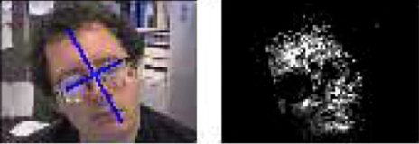
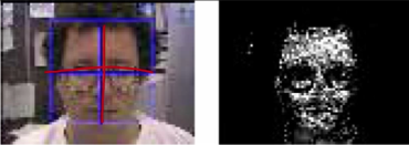
Visual Tracking
Conventional approaches
- Build a model before tracking starts
- Use contours, color, or appearance to represent an object
- Then do one of:
- Optical flow
- Patch tracking with particles
- Solve complicated optimization problem
- Incorporate invariance to cope with variation in pose, lighting, view angle...
- Problem:
- Object appearance and environments are always changing
A few key inspirations:
- Eigentracking [Black and Jepson 96]
- View-based learning method
- Learn to track a "thing" rather than some "stuff"
- Key insight: seperate geometry from appearance - use deformable model
- But...need to solve nonlinear optimization problem
- And fixed basis set
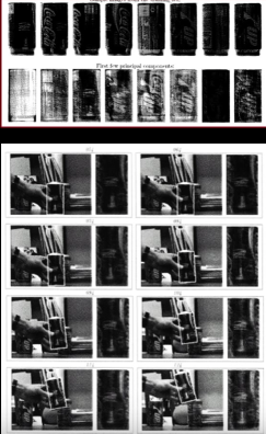
Fig 22(a)
- Active contour [Isard and Blake]
- Use particle filter
- Propagate uncertainty over time
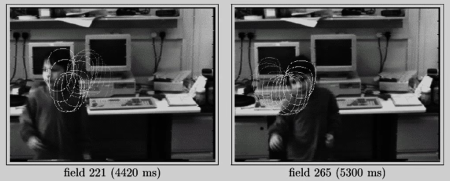
Incremental Visual Learning
- Aim to build a tracker that:
- Is not single image based
- Constantly updates the model
- Learns a representation while tracking
- Runs fast
- Operates on moving camera
- Challenge
- Pose variation
- Partial occlusion
- Illumination change
- Drifts
Main idea
- Adaptive visual tracker:
- Particle filter -draw samples from distributions of deformation
- Subspace-based tracking
- Learn to track the "thing" - like the face in eigenfaces
- Use it to determine the most likely sample
- Incremental subspace update
- Does not need to build the model prior to tracking
- Handles variations in lighting, pose (and expression)
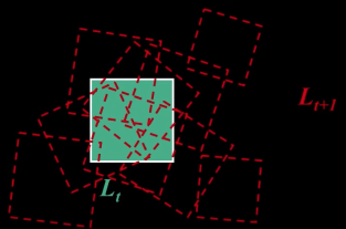
For Sampling-Based Method
Nomenclature
- Location at time $\color{blue}{t:L_t}$
- Current observation: $\color{blue}{F_t}$
Goal: Predict target location $\color{blue}{L_t}$ based on $\color{blue}{L_{t-1}}$ (location in last frame)
$$\color{blue}{p(L_t|F_t,L_{t-1})\propto} \color{#00cccc}{p(F_t|L_t)}\cdot \color{#990099}{p(L_t|L_{t-1})}$$
- $\color{#990099}{p(L_t|L_{t-1})} \rightarrow$ dynamics model
- Here use Brownian motion to model the dynamics - no velocity model
- $\color{#00cccc}{p(F_t|L_t)}\rightarrow$ observation model
- Use eigenbasis with approximation
Dynamic Model
Dynamic Model $L_t$
Representation of $\color{blue}{L_t}$
- similarity transform: Position $\color{blue}{x_t,y_t}$, rotation $\color{blue}{\theta_t}$, scaling $\color{blue}{s_t}$
- 4 parameters
Or,
- Affine tranform with 6 parameters
Dynamic Model $p(L_t|L_{t-1}$
Simple dynamics model:
- Each parameter is independently Gaussian distributed
$$\color{blue}{p(L_t|L_0) = N(x_1;x_0;\sigma^2_x)N(y_1;y_0;\sigma^2_y)N(\theta_1;\theta_0;\sigma^2_\theta)N(s_1;s_0;\sigma^2_s)}$$
Observation Model
Observation Model: $p(F_t|L_t)$
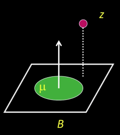
Use probabilistic principal component analysis (PPCA) to model our image observation process
Given a location $\color{blue}{L_t}$, assume the observed frame was generated from the eigenbasis
The probability of observing a datum $\color{blue}{z}$ given the eigenbasis $\color{blue}{B}$ and mean $\color{blue}{\mu}$,
$$\color{blue}{p(z|B) = N(z;\mu,BB^T + \epsilon I)}$$
where $\color{blue}{\epsilon I}$ is additive Gaussian noise
In the limit $\color{blue}{\epsilon \rightarrow 0}$:
$\color{blue}{p(z|B) = N(z;\mu,BB^T + \epsilon I)}$ is mostly a function of the distance between $\color{blue}{z}$ and the linear subspace $\color{blue}{B}$
$$\color{blue}{p(z|B) \propto exp(-||(z-\mu) -}\color{#990099}{BB^T(z-\mu)}\color{blue}{||^2)}$$
where:
$\color{#990099}{BB^T(z-\mu)}$: reconstruction
Why is that the reconstruction?
$\color{#990099}{B^T}$ is (small) $\color{#990099}{k}$ $x$ (big) $\color{#990099}{d}$
$\color{#990099}{B^T(z-\mu)}$ is the coefficient vector (say $\color{#990099}{\gamma}$) of $\color{#990099}{z-\mu}$
Then $\color{#990099}{B\gamma}$ is the reconstruction
Incremental Subspace Update
The cool part...
Do not assume the observation model remains fixed over time
- We allow for incremental update of our object model
Given inital eigenbasis $\color{blue}{B_{t-1}}$ and new observation $\color{blue}{w_{t-1}}$, compute a new eigenbasis $\color{blue}{B_t}$
$\color{blue}{B_t}$ is then used in $\color{blue}{p(F_t|L_t)}$
Why? To account for appearance change due to pose, illumination, shape variation.
- Learn and appearance representation while tracking
- Based on the R-SVD algorithm [Golub and Van Loan 96] and the sequential Karhunen-Loeve algorithm [Levy and Lindebaum 00]
- Essentially: Develop an update algorithm with respect to running mean, allowing for decay
Put All Together
- (Optional) Construct an initial eigenbasis if necessary (e.g., for inital detection)
- Choose initial location $\color{blue}{L_0}$
- Generate possible locations: $\color{blue}{p(L_t|L_{t-1})}$
- Evaluate possible locations: $\color{blue}{p(F_t|L_{t-1})}$
- Select the most likely location by Bayes: $\color{blue}{p(L_t|F_t,L_{t-1})}$
- Update eigenbasis using R-SVD algorithm
- Go to step 3
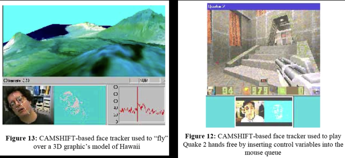
Experiments
- 30 frame per second with $320 \times 240$ pixel resolution on old machines...
- Draw at most 500 samples
- 50 eigenvectors
- Update every 5 frames
- Runs XXX(<2 & >1000) frames per second using Matlab

Occlusion Handling
Most Recent Work
- Handling occlusion
An iterative method to compute a weight mask
- Estimate the probability a pixel is being occluded
Given an observation $\color{blue}{l_t}$, initially assume there is no occlusion with $\color{blue}{W^0}$
$$\color{blue}{D^{(i)} = W^{(i)}\cdot *(I_t - UU^TI_t)}$$
$$\color{blue}{W^{(i+1)} = exp \left (\frac{-D^{(i)^2}}{\sigma^2}\right )}$$
where $\color{blue}{\cdot *}$ is element-wise multiplication
Implementation of Incremental Learning for Robust Visual Tracking is available at
https://github.com/kuhess/ultraking
But outdated
Remember: Supervised classification
Given a collection of labeled examples, come up with a function that will predict the labels of new examples
Supervised classification
Since we know the desired labels of training data, we want to minimize the expected misclassification
Two general strategies:
- Generative - probabilistically model the classes
- Discriminative - probabilistically model the decision (the boundaries)
Generative Classification and Minimal Risk
Review Minimal Risk above
Some Challenges for Generative Models
Generative approaches were some of the first methods in pattern recognition
- Easy to model analytically and could be done with modest amounts of moderate dimenstional data
But for the modern world there are some liabilties:
- Many signals are high-dimensional and representing the complete density of class is data-hard
- In some sense, we don't care about modeling the classes, *we only care about making the right decisions.
- Model the hard cases- the ones near the boundaries!!
- We don't typically know which features of instances actually discriminate between classes
Discriminative Classification Assumptions
Going forward we're going to make some assumptions
- There are a fixed number of known classes.
- Ample number of training examples of each class.
- Equal cost of making mistakes - what matters is getting the label right.
- Need to construct a representation of the instance but we don't know a priori what features are diagnostic of the class label
Basic Framework
Train
- Build an object model - representation
Describe training instances (here images) - Learn/train a classifier
Test
- Generate candidates in new image
- Score the candidates
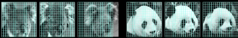
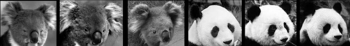
Window Based Models
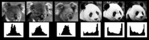
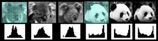
Simple holistic descriptions of image content
- Grayscale/ color histogram
vector of pixel intensities
Pixel-based representations sensitive to small shifts
Color or grayscale-based description can be sensitive to illumination and intra-class appearance variation
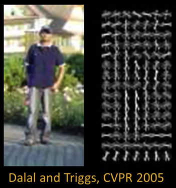
Consider edges, contours, and (oriented) intensity gradients
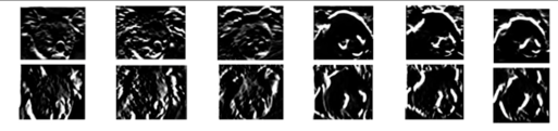
Summarize local distribution of gradients with histogram
- Locally orderless: offers invariance to small shifts and rotations
- Contrast-normalization: try to correct for variable illumination


Window Based Object Detection

Training:
- Obtain training data
- Define features
- Train classifier
Given new image:
- Slide window
- Score by classifier
Nearest Neighbor
Discriminative classification methods
Discriminative classifiers -find a division (surface) in feature space that separates the classes
Several methods:
- Nearest neighbors
- Boosting
- Support Vector Machines
Nearest Neighbor classification
Choose label of nearest training data point
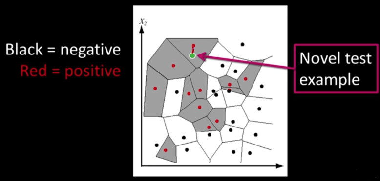
Voronoi partitioning of feature space for 2-category 2D data
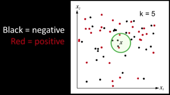
K-Nearest Neighbors classification
- For a new point, find the k closest points from training data
- Labels of the k points "vote" to classify
"""
===============
Demo K-NN: Tabular data
Source: https://machinelearningmastery.com/tutorial-to-implement-k-nearest-neighbors-in-python-from-scratch/
===============
"""
import csv
import random
import math
import operator
def loadDataset(filename, split, trainingSet=[] , testSet=[]):
with open(filename, 'rb') as csvfile:
lines = csv.reader(open(filename, "r"))
dataset = [l for l in lines]
for x in range(len(dataset)-1):
for y in range(4):
dataset[x][y] = float(dataset[x][y])
if random.random() < split:
trainingSet.append(dataset[x])
else:
testSet.append(dataset[x])
def euclideanDistance(instance1, instance2, length):
distance = 0
for x in range(length):
distance += pow((instance1[x] - instance2[x]), 2)
return math.sqrt(distance)
def getNeighbors(trainingSet, testInstance, k):
distances = []
length = len(testInstance)-1
for x in range(len(trainingSet)):
dist = euclideanDistance(testInstance, trainingSet[x], length)
distances.append((trainingSet[x], dist))
distances.sort(key=operator.itemgetter(1))
neighbors = []
for x in range(k):
neighbors.append(distances[x][0])
return neighbors
def getResponse(neighbors):
classVotes = {}
for x in range(len(neighbors)):
response = neighbors[x][-1]
if response in classVotes:
classVotes[response] += 1
else:
classVotes[response] = 1
sortedVotes = sorted(classVotes.items(), key=operator.itemgetter(1), reverse=True)
return sortedVotes[0][0]
def getAccuracy(testSet, predictions):
correct = 0
for x in range(len(testSet)):
if testSet[x][-1] == predictions[x]:
correct += 1
return (correct/float(len(testSet))) * 100.0
def main():
# prepare data
trainingSet=[]
testSet=[]
split = 0.67
loadDataset('iris.data', split, trainingSet, testSet)
print('Train set: ' + repr(len(trainingSet)))
print('Test set: ' + repr(len(testSet)))
# generate predictions
predictions=[]
k = 3
for x in range(len(testSet)):
neighbors = getNeighbors(trainingSet, testSet[x], k)
result = getResponse(neighbors)
predictions.append(result)
print('> predicted=' + repr(result) + ', actual=' + repr(testSet[x][-1]))
accuracy = getAccuracy(testSet, predictions)
print('Accuracy: ' + repr(accuracy) + '%')
main()
"""
===============
Demo K-NN: Image data
Source: https://gurus.pyimagesearch.com/lesson-sample-k-nearest-neighbor-classification/
===============
"""
from __future__ import print_function
from sklearn.neighbors import KNeighborsClassifier
from sklearn.metrics import classification_report
from sklearn import datasets
from skimage import exposure
import numpy as np
import imutils
import cv2
import sklearn
# handle older versions of sklearn
if int((sklearn.__version__).split(".")[1]) < 18:
from sklearn.cross_validation import train_test_split
# otherwise we're using at lease version 0.18
else:
from sklearn.model_selection import train_test_split
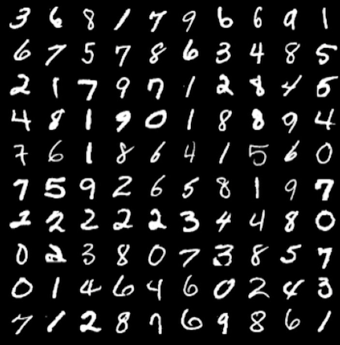
# load the MNIST digits dataset
mnist = datasets.load_digits()
# take the MNIST data and construct the training and testing split, using 75% of the
# data for training and 25% for testing
(trainData, testData, trainLabels, testLabels) = train_test_split(np.array(mnist.data),
mnist.target, test_size=0.25, random_state=42)
# now, let's take 10% of the training data and use that for validation
(trainData, valData, trainLabels, valLabels) = train_test_split(trainData, trainLabels,
test_size=0.1, random_state=84)
# show the sizes of each data split
print("training data points: {}".format(len(trainLabels)))
print("validation data points: {}".format(len(valLabels)))
print("testing data points: {}".format(len(testLabels)))
# initialize the values of k for our k-Nearest Neighbor classifier along with the
# list of accuracies for each value of k
kVals = range(1, 30, 2)
accuracies = []
# loop over various values of `k` for the k-Nearest Neighbor classifier
for k in range(1, 30, 2):
# train the k-Nearest Neighbor classifier with the current value of `k`
model = KNeighborsClassifier(n_neighbors=k)
model.fit(trainData, trainLabels)
# evaluate the model and update the accuracies list
score = model.score(valData, valLabels)
print("k=%d, accuracy=%.2f%%" % (k, score * 100))
accuracies.append(score)
# find the value of k that has the largest accuracy
i = int(np.argmax(accuracies))
print("k=%d achieved highest accuracy of %.2f%% on validation data" % (kVals[i],
accuracies[i] * 100))
# re-train our classifier using the best k value and predict the labels of the
# test data
model = KNeighborsClassifier(n_neighbors=kVals[i])
model.fit(trainData, trainLabels)
predictions = model.predict(testData)
# show a final classification report demonstrating the accuracy of the classifier
# for each of the digits
print("EVALUATION ON TESTING DATA")
print(classification_report(testLabels, predictions))
# loop over a few random digits
for i in list(map(int, np.random.randint(0, high=len(testLabels), size=(5,)))):
# grab the image and classify it
image = testData[i]
prediction = model.predict(image.reshape(1, -1))[0]
# convert the image for a 64-dim array to an 8 x 8 image compatible with OpenCV,
# then resize it to 32 x 32 pixels so we can see it better
image = image.reshape((8, 8)).astype("uint8")
image = exposure.rescale_intensity(image, out_range=(0, 255))
image = imutils.resize(image, width=32, inter=cv2.INTER_CUBIC)
# show the prediction
print("I think that digit is: {}".format(prediction))
cv2.imshow("Image", image)
cv2.waitKey(0)

Viola Jones Face Detector Introduction
Viola-Jones face detector
Main ideas:
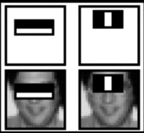
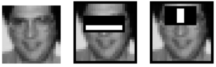
- Represent brightness patterns with efficiently computable "rectangular" features within window of interest
Viola-Jones face detector: Features

Viola-Jones face detector: Integral Image

Computing Sum Within a Rectangle
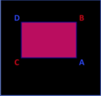
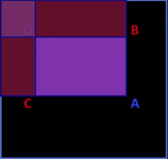
- Let A, B, C, D be the values of the integral image at the corners of a rectangle
- Then the sum of original image values within the rectangle can be computed as
$$\color{#990099}{sum} = \color{blue}{A}-\color{red}{B} - \color{red}{C} + \color{blue}{D}$$
- Only 3 additions are required for any size of rectangle
Avoid scaling images
$\rightarrow$ scale features directly for same cost
## Computing integral image python
import numpy as np
import cv2
from matplotlib import pyplot as plt
import PIL
from io import BytesIO
from IPython.display import clear_output, Image as NoteImage, display
def imshow(im,fmt='jpeg'):
#a = np.uint8(np.clip(im, 0, 255))
f = BytesIO()
PIL.Image.fromarray(im).save(f, fmt)
display(NoteImage(data=f.getvalue()))
def imread(filename):
img = cv2.imread(filename)
img = cv2.cvtColor(img, cv2.COLOR_BGR2RGB)
return img
def gray(im):
return cv2.cvtColor(im.copy(), cv2.COLOR_BGR2GRAY)
def to_integral(img: np.ndarray) -> np.ndarray:
integral = np.cumsum(np.cumsum(img, axis=0), axis=1)
return np.pad(integral, (1, 1), 'constant', constant_values=(0, 0))[:-1, :-1]
snap = imread("imgs/messimadrid.jpg")
imshow(snap)
snapg = gray(snap)
x1=50; y1=280
x2=350; y2 = 400
I = cv2.integral( snapg )
I = to_integral(snapg)
window = snapg[x1:x2, y1:y2]
imshow(window)
print("Sum from the image %d" % sum(window.flatten()))
print("Sum from the integral image %d" % (I[x2,y2]-I[x1,y2] - I[x2,y1]+I[x1,y1]))


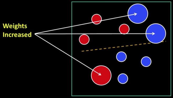
Weak Learners
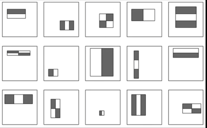
Considering all possible filter parameters -position, scale, and type:
180,000+ possible features associated with each 24 x 24 window
Viola-Jones face detector
Main ideas:
- Represent brightness patterns with efficiently computable "rectangular" features within window of interest
- Choose discriminative features to be weak classifiers/learners

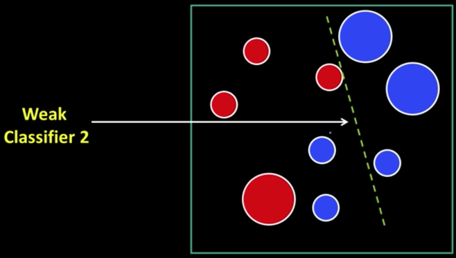
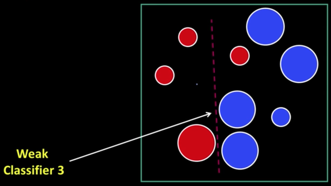
Cascade
Main ideas:
- Represent brightness patterns with efficiently computable "rectangular" features within window of interest
- Choose discriminative features to be weak classifiers/learners
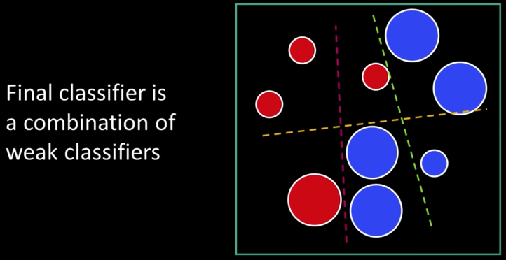
- Use boosted combination of them as final classifier
- Form a cascade of such classifiers, rejecting clear negatives quickly</font>
$2^{nd}$ big idea: Cascade...
Even if the filters are fast to compute, each new image has a lot of possible window to search
How to make the detection more efficient?
Key insight: almost every where is a non-face
- So... detect non-faces more quickly than faces.
- And if you say it's not a face, be sure and move on
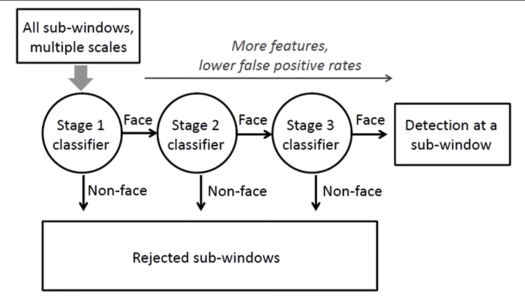
- Form a cascade with really low false negative rates early
- At each stage use the false positives from last stage as "difficult negatives*
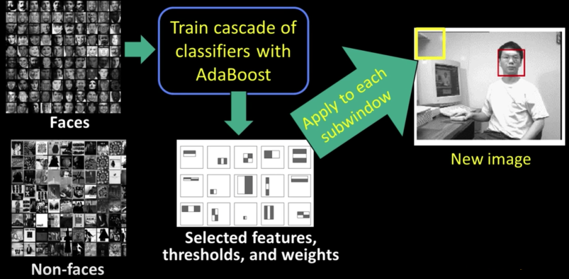
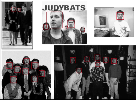
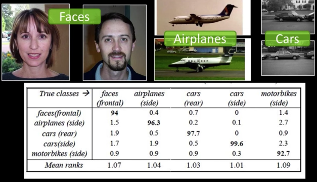
Viola-Jones detector: Summary
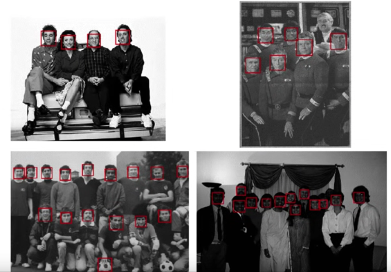
Viola-Jones detector: Results

Detecting profile faces
*Can we use the same detector?
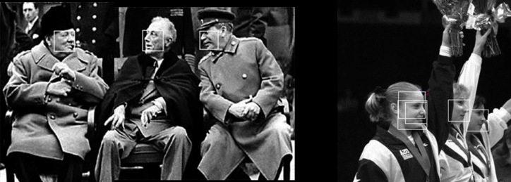
Example using Viola-Jones detector

Consumer applications: iPhoto 2009
Summary
Key ideas:
- Rectangular features and integral image
- AdaBoost for feature selection
- Cascade
Training is slow, but detection is very fast
Really, really effective...
Boosting (general): Advantages
- Integrates classification with feature selection
- Flexibility in the choice of weak learners, boosting scheme
- Complexity of training is linear in the number of training examples
- Testing is fast
- Easy to implement
Boosting: Disadvantages
- Needs many training examples
- Often found not to work as well as an alternative discriminative classifier, support vector machine (SVM)
- Especially for many-class problems
import numpy as np
import cv2 as cv
face_cascade = cv.CascadeClassifier('haarcascade_frontalface_default.xml')
eye_cascade = cv.CascadeClassifier('haarcascade_eye.xml')
imgs_files = ["imgs/messigold.jpg",'imgs/barca.jpg','imgs/messimadrid.jpg']
imgs = [imread(i) for i in imgs_files]
grays = [gray(i) for i in imgs]
for i,g in enumerate(grays):
img = imgs[i]
faces = face_cascade.detectMultiScale(g, 1.3, 5)
for (x,y,w,h) in faces:
cv.rectangle(img,(x,y),(x+w,y+h),(255,0,0),2)
roi_gray = g[y:y+h, x:x+w]
roi_color = img[y:y+h, x:x+w]
eyes = eye_cascade.detectMultiScale(roi_gray)
for (ex,ey,ew,eh) in eyes:
cv.rectangle(roi_color,(ex,ey),(ex+ew,ey+eh),(0,255,0),2)
imshow(img)


Checkout Markus Mayer notebook on Viola-Jones
We used Mayer notebook for creating weak classifiers. Below we load it and test it. If you wish to train your own, please use Mayer notebook
In order to use the classifiers, we need to copy some utility functions, classes and global variables
Utility Functions
import pickle
from typing import *
from numba import jit
from PIL import Image, ImageOps
import numpy as np
WINDOW_SIZE = 15
sample_mean = 0.6932713985443115
sample_std = 0.18678635358810425
HALF_WINDOW = WINDOW_SIZE // 2
def gleam(values: np.ndarray) -> np.ndarray:
return np.sum(gamma(values), axis=2) / values.shape[2]
def gamma(values: np.ndarray, coeff: float=2.2) -> np.ndarray:
return values**(1./coeff)
def normalize_weights(w: np.ndarray) -> np.ndarray:
return w / w.sum()
def to_integral(img: np.ndarray) -> np.ndarray:
integral = np.cumsum(np.cumsum(img, axis=0), axis=1)
return np.pad(integral, (1, 1), 'constant', constant_values=(0, 0))[:-1, :-1]
def to_float_array(img: Image.Image) -> np.ndarray:
return np.array(img).astype(np.float32) / 255.
def to_image(values: np.ndarray) -> Image.Image:
return Image.fromarray(np.uint8(values * 255.))
def normalize(im: np.ndarray, mean: float = sample_mean, std: float = sample_std) -> np.ndarray:
return (im - mean) / std
def load_image(imgFile):
original_image = Image.open(imgFile)
target_size = (384, 288)
thumbnail_image = original_image.copy()
thumbnail_image.thumbnail(target_size, Image.ANTIALIAS)
thumbnail_image
original = to_float_array(thumbnail_image)
grayscale = gleam(original)
return thumbnail_image,grayscale
Classes
WeakClassifier = NamedTuple('WeakClassifier', [('threshold', float), ('polarity', int),
('alpha', float),
('classifier', Callable[[np.ndarray], float])])
class Feature:
def __init__(self, x: int, y: int, width: int, height: int):
self.x = x
self.y = y
self.width = width
self.height = height
def __call__(self, integral_image: np.ndarray) -> float:
try:
return np.sum(np.multiply(integral_image[self.coords_y, self.coords_x], self.coeffs))
except IndexError as e:
raise IndexError(str(e) + ' in ' + str(self))
def __repr__(self):
return f'{self.__class__.__name__}(x={self.x}, y={self.y}, width={self.width}, height={self.height})'
class Feature4(Feature):
def __init__(self, x: int, y: int, width: int, height: int):
super().__init__(x, y, width, height)
hw = width // 2
hh = height // 2
self.coords_x = [x, x + hw, x, x + hw, # upper row
x + hw, x + width, x + hw, x + width,
x, x + hw, x, x + hw, # lower row
x + hw, x + width, x + hw, x + width]
self.coords_y = [y, y, y + hh, y + hh, # upper row
y, y, y + hh, y + hh,
y + hh, y + hh, y + height, y + height, # lower row
y + hh, y + hh, y + height, y + height]
self.coeffs = [1, -1, -1, 1, # upper row
-1, 1, 1, -1,
-1, 1, 1, -1, # lower row
1, -1, -1, 1]
class Feature2h(Feature):
def __init__(self, x: int, y: int, width: int, height: int):
super().__init__(x, y, width, height)
hw = width // 2
self.coords_x = [x, x + hw, x, x + hw,
x + hw, x + width, x + hw, x + width]
self.coords_y = [y, y, y + height, y + height,
y, y, y + height, y + height]
self.coeffs = [1, -1, -1, 1,
-1, 1, 1, -1]
class Feature2v(Feature):
def __init__(self, x: int, y: int, width: int, height: int):
super().__init__(x, y, width, height)
hh = height // 2
self.coords_x = [x, x + width, x, x + width,
x, x + width, x, x + width]
self.coords_y = [y, y, y + hh, y + hh,
y + hh, y + hh, y + height, y + height]
self.coeffs = [-1, 1, 1, -1,
1, -1, -1, 1]
class Feature3h(Feature):
def __init__(self, x: int, y: int, width: int, height: int):
super().__init__(x, y, width, height)
tw = width // 3
self.coords_x = [x, x + tw, x, x + tw,
x + tw, x + 2*tw, x + tw, x + 2*tw,
x + 2*tw, x + width, x + 2*tw, x + width]
self.coords_y = [y, y, y + height, y + height,
y, y, y + height, y + height,
y, y, y + height, y + height]
self.coeffs = [-1, 1, 1, -1,
1, -1, -1, 1,
-1, 1, 1, -1]
class Feature3v(Feature):
def __init__(self, x: int, y: int, width: int, height: int):
super().__init__(x, y, width, height)
th = height // 3
self.coords_x = [x, x + width, x, x + width,
x, x + width, x, x + width,
x, x + width, x, x + width]
self.coords_y = [y, y, y + th, y + th,
y + th, y + th, y + 2*th, y + 2*th,
y + 2*th, y + 2*th, y + height, y + height]
self.coeffs = [-1, 1, 1, -1,
1, -1, -1, 1,
-1, 1, 1, -1]
@jit
def run_weak_classifier(x: np.ndarray, c: WeakClassifier) -> float:
return weak_classifier(x=x, f=c.classifier, polarity=c.polarity, theta=c.threshold)
@jit
def weak_classifier(x: np.ndarray, f: Feature, polarity: float, theta: float) -> float:
# return 1. if (polarity * f(x)) < (polarity * theta) else 0.
return (np.sign((polarity * theta) - (polarity * f(x))) + 1) // 2
@jit
def strong_classifier(x: np.ndarray, weak_classifiers: List[WeakClassifier]) -> int:
sum_hypotheses = 0.
sum_alphas = 0.
for c in weak_classifiers:
sum_hypotheses += c.alpha * run_weak_classifier(x, c)
sum_alphas += c.alpha
return 1 if (sum_hypotheses >= .5*sum_alphas) else 0
Predict and Display Functions
def predict(img,classifiers):
normalized_integral = to_integral(normalize(img))
rows, cols = normalized_integral.shape[0:2]
face_positions_1 = []
face_positions_2 = []
face_positions_3 = []
for row in range(HALF_WINDOW + 1, rows - HALF_WINDOW):
for col in range(HALF_WINDOW + 1, cols - HALF_WINDOW):
window = normalized_integral[row-HALF_WINDOW-1:row+HALF_WINDOW+1, col-HALF_WINDOW-1:col+HALF_WINDOW+1]
# First cascade stage
probably_face = strong_classifier(window, classifiers[0])
if probably_face < .5:
continue
face_positions_1.append((row, col))
# Second cascade stage
probably_face = strong_classifier(window, classifiers[1])
if probably_face < .5:
continue
face_positions_2.append((row, col))
# Third cascade stage
probably_face = strong_classifier(window, classifiers[2])
if probably_face < .5:
continue
face_positions_3.append((row, col))
print(f'Found {len(face_positions_1)} candidates at stage 1, {len(face_positions_2)} at stage 2 and {len(face_positions_3)} at stage 3.')
return face_positions_1,face_positions_2, face_positions_3
def render_candidates(image: Image.Image, candidates: List[Tuple[int, int]]) -> Image.Image:
canvas = to_float_array(image.copy())
for row, col in candidates:
canvas[row-HALF_WINDOW-1:row+HALF_WINDOW, col-HALF_WINDOW-1, :] = [1., 0., 0.]
canvas[row-HALF_WINDOW-1:row+HALF_WINDOW, col+HALF_WINDOW-1, :] = [1., 0., 0.]
canvas[row-HALF_WINDOW-1, col-HALF_WINDOW-1:col+HALF_WINDOW, :] = [1., 0., 0.]
canvas[row+HALF_WINDOW-1, col-HALF_WINDOW-1:col+HALF_WINDOW, :] = [1., 0., 0.]
return to_image(canvas)
Loading the classifiers
clsf_files = [
["vj_model/1st-weak-learner-%d-of-2.pickle" % i for i in range(1,3)],
["vj_model/2nd-weak-learner-%d-of-10.pickle" % i for i in range(1,11)],
["vj_model/3rd-weak-learner-%d-of-25.pickle" % i for i in range(1,26)]
]
classifiers = [[],[],[]]
for i,s in enumerate(clsf_files):
for f in s:
file = open(f,'rb')
wk_class = pickle.load(file)
classifiers[i].append(wk_class)
file.close()
imgs_files = ['imgs/messimadrid.jpg',"imgs/messigold.jpg",'imgs/barca.jpg']
for img in imgs_files:
cimg,gimg = load_image(img)
pos1,pos2,pos3 = predict(gimg,classifiers)
imshow(np.array(render_candidates(cimg,pos3)))


Linear classifiers

Lines in $R^2$

$$\color{blue}{w = \begin{bmatrix}p\\q\end{bmatrix}\,\,\,x = \begin{bmatrix}p\\q\end{bmatrix}}$$
$$\color{blue}{px + qy + b = 0}$$
$$\color{#75e9fe}{w\cdot x + b=0}$$
$$\text{Distance from point to line}\,\,\,\color{blue}{D = \frac{|px_0+qy_0+b|}{\sqrt{p^2+q^2}}=\frac{w^Tx + b}{|w|}}$$
SVMs
Find linear function to seperate positive and negative examples
$\color{blue}{x_i}$ positive: $\,\,\,\color{blue}{x_i\cdot w + b\ge0}$
$\color{blue}{x_i}$ negative: $\,\,\,\color{blue}{x_i\cdot w + b < 0}$

Discriminative classifier based on optimal separating line (2D case)
Maximize the margin between the positive and negative training examples

How to maximize the margin?
$\color{blue}{x_i}$ positive$\color{blue}{y_i=1}$: $\,\,\,\color{blue}{x_i\cdot w + b\ge0}$
$\color{blue}{x_i}$ negative$\color{blue}{y_i=-1}$: $\,\,\,\color{blue}{x_i\cdot w + b < 0}$
For support vectors, $\color{blue}{x_i\cdot w + b \pm 1}$
Dist. between point and line: $\color{blue}{\frac{|x_i\cdot w + b|}{||w||}}$
For support vectors: $\color{blue}{\frac{w^Tx+b}{||w||}=\frac{\pm 1}{||w||}}$
$$\color{blue}{M = \left | \frac{1}{||w||} - \frac{-1}{||w||}\right | = \frac{2}{||w||}}$$

Finding the Maximum Margin Line
- Maximize margin $\color{blue}{\frac{2}{||w||}}$
- Correctly classify all training data points:
$\;\;\;\;\;\;\;\; \color{blue}{x_i}$ positive$\color{blue}{y_i=1}$: $\,\,\,\color{blue}{x_i\cdot w + b\ge1}$
$\;\;\;\;\;\;\;\; \color{blue}{x_i}$ negative$\color{blue}{y_i=-1}$: $\,\,\,\color{blue}{x_i\cdot w + b \le -1}$
- Quadratic optimization problem:
$$\text{Minimize}\,\,\color{blue}{\frac{1}{2}w^Tw}$$
$$\text{Subject to}\,\,\color{blue}{y_i(x_i\cdot w + b)\ge 1}$$
Solution: $\;\;\;\; \color{blue}{w = \sum_i \alpha_iy_ix_i}$
where:
$\color{blue}{x_i}\,\,\text{: support vector}$
$\color{blue}{\alpha_i}\,\,\text{: learned weight}$
The weights $\color{blue}{\alpha_i}$ are non-zero only at support vectors
So:
$$\color{blue}{w = \sum_i \alpha_iy_ix_i}$$
$$\color{blue}{b = y_i-w\cdot x_i}\,\,\,\,\text{(for any support vector)}$$
$$\color{blue}{w\cdot x + b = \sum_i \alpha_iy_ix_i \cdot x + b}$$
Classification function:
$$\color{blue}{f(x) = sign(w\cdot x + b)}$$
$$\color{blue}{f(x) = sign \left (\sum_i \alpha_i x_i \cdot x + b\right )}$$
if $\color{blue}{f(x) < 0}$, classify as negative
if $\color{blue}{f(x) > 0}$, classify as positive
Questions
- What if the features are not 2D?
- Generalizes to d-dimensions
- Replace line with hyperplane
- What if the data is not linearly separable?
- What if we have more than just two categories?

Non Linear SVMs
What if the data is not linearly separable?
- Datasets that are linearly separable with some noise work out great:
But what are we going to do if the dataset is just too hard?
How about... mapping data to a higher-dimensional space
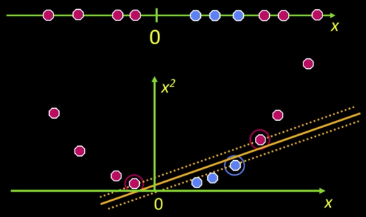
- General idea: Original input space can be mapped to some higher-dimensional feature space...
The Kernel Trick
We saw linear classifier relies on dot product between vectors.
Define:
$$\color{blue}{K(x_i,x_j) = x_i\cdot x_j = x_i^Tx_j}$$
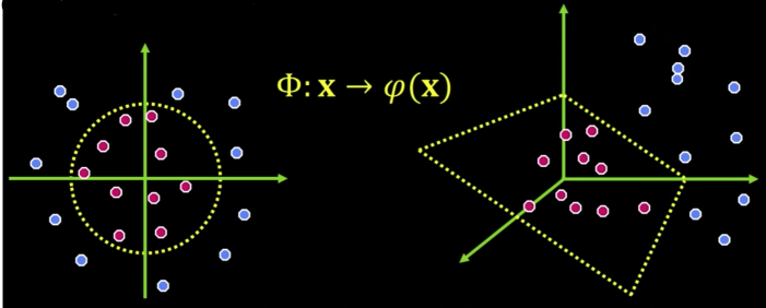
If every data point is mapped into high-dimensional space via some transformation
$$\color{blue}{\Phi = x \rightarrow \varphi(x)}$$
the dot product becomes:
$$\color{blue}{K(x_i,x_j) = \varphi(x_i)^T\varphi(x_j)}$$
A kernel function is a "similarity" function that corresponds to an inner product in some expanded feature space
Example
E.g.,
2D vectors $\color{blue}{x=\begin{bmatrix}x_1&x_2\end{bmatrix}}$
Let
$$\color{blue}{K(x_i,x_j) = (1+x_i^Tx_j)^2}$$
We need to show that $\color{blue}{K(x_i,x_j) = \varphi(x_i)^T\varphi(x_j)$:
$$\color{blue}{K(x_i,x_j) = (1+x_i^Tx_j)^2}$$
$$\color{blue}{=1+x_{i1}^2x_{j1}^2 + 2x_{i1}x_{j1}x_{i2}x_{j2}+x_{i2}^2x_{j2}^2+2x_{i1}x_{j1}+2x_{i2}x_{j2}}$$
$$\color{blue}{=}\color{#42d4f4}{\begin{bmatrix}1&x^2_{i1}&\sqrt{2}x_{i1}x_{i2}&x^2_{i2}&\sqrt{2}x_{i1}&\sqrt{2}x_{i2}\end{bmatrix}}\color{blue}{^T}\color{#b841f4}{\begin{bmatrix}1&x^2_{j1}&\sqrt{2}x_{j1}x_{j2}&x^2_{j2}&\sqrt{2}x_{j1}&\sqrt{2}x_{j2}\end{bmatrix}}$$
$$\color{blue}{=}\color{#42d4f4}{\varphi(x_i)}\color{blue}{^T}\color{#b841f4}{\varphi(x_j)}$$
Where $\color{blue}{\varphi(x) = \begin{bmatrix}1&x^2_{1}&\sqrt{2}x_{1}x_{2}&x^2_{2}&\sqrt{2}x_{1}&\sqrt{2}x_{2}\end{bmatrix}}$
Nonlinear SVMs
The kernel trick: Instead of explicitly computing the lifting transformation $\color{blue}{\varphi(x)}$, define a kernel function $\color{blue}{K}$:
$$\color{blue}{K(x_i,x_j) = \varphi(x_i)^T\varphi(x_j)}$$
This gives a nonlinear decision boundary in the original feature space:
$$\color{blue}{\sum_i \alpha_iy_i(x_i^Tx) + b \rightarrow \sum_i \alpha_iy_iK(x_i,x) + b}$$
Examples of Kernel Functions
- Linear $\color{blue}{K(x_i,x_j) = x_i^Tx_j}$
- Number of dimensions: N (just size of x)
Gaussian RBF $\color{blue}{K(x_i,x_j) = exp\left (-\frac{||x_i-x_j||^2}{2\sigma^2}\right )}$
Number of dimesnsions: Infinite
$\color{blue}{exp\left (-\frac{1}{2}||x-x'||^2_2\right ) = \sum_{j=0}^\color{#b841f4}{\infty}\frac{(x^Tx')^j}{j!}exp\left (-\frac{1}{2}||x||^2_2\right )exp\left (-\frac{1}{2}||x'||^2_2\right )}$
- Historgram intersection
$$\color{blue}{K(x_i,x_j) = \sum_k min(x_i(k),x_j(k))}$$
- Number of dimensions: Large. See: [Alexander C. Berg, Jitendra Malik, "Classification using intersection kernel support vector machines is efficient", CVPR,2008]X = [[181, 80, 44], [177, 70, 43], [160, 60, 38],
[154, 54, 37],[166, 65, 40], [190, 90, 47], [175, 64, 39],
[177, 70, 40], [159, 55, 37], [171, 75, 42],
[181, 85, 43], [168, 75, 41], [168, 77, 41]]
Y = ['male', 'male', 'female', 'female', 'male', 'male',
'female','female','female', 'male', 'male',
'female', 'female']
test_data = [[190, 70, 43],[154, 75, 38],[181,65,40]]
test_labels = ['male','female','male']
from sklearn.svm import SVC
#Support Vector Classifier
print("Ground Truth",test_labels)
kernels = ['linear', 'poly', 'rbf', 'sigmoid']
for k in kernels:
s_clf = SVC(kernel=k)
s_clf.fit(X,Y)
s_prediction = s_clf.predict(test_data)
print(k,s_prediction)
## checkout this gender recognition from voice
## https://github.com/deeshashah/python-gender-recognition
SVM for recognition: Training
Training
- Define your representation
- Select a kernel function
- Compute pairwise kernel values between labeled examples
- Use this "kernel matrix" to solve for SVM support vectors & weights
Recognition
To classify a new example:
- Compute kernel values between new input and support vectors
- Apply weights
- Check sign of output

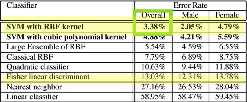
Learning Gender with SVMs

- Training examples : 1044 males, 713 females
- Images reduced to 21x12(!!)
- Experiment with various kernels, select Gaussian RBF
$$\color{blue}{K(x_i,x_j) = exp\left (-\frac{||x_i-x_j||^2}{2\sigma^2}\right )}$$
When computing new input x
$$\color{blue}{K(\color{#b841f4}{x},x_j) = exp\left (-\frac{||\color{#b841f4}{x}-x_j||^2}{2\sigma^2}\right )}$$
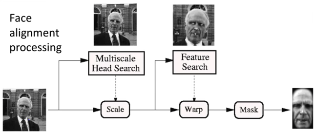
Support faces

Gender perception experiment: How well can humans do?
Subjects:
- 30 people (22 male, 8 female), ages mid-20's to mid-40's
Test data:
- 254 face images (60% males, 40% females)
- Low res and high res versions
Task:
- Classify as male or female, forced choice
- No time limit


"""
Data source: http://pics.psych.stir.ac.uk/zips/nottingham.zip
100 face images
Similar to the link below, we used face_recognition module to create features. Check face_gender/make_dataset.py
https://github.com/cftang0827/face_gender
You might need to unzip the file face_gender/nottingham.zip first
"""
import matplotlib.pyplot as plt
from os import listdir
from os.path import isfile, join
from PIL import Image, ImageOps
files = [join("face_gender/nottingham", f) for f in listdir("face_gender/nottingham") if isfile(join("face_gender/nottingham", f))]
imgs = [Image.open(f).convert('RGB') for f in files]
f,ax = plt.subplots(10,10)
f.set_size_inches((15,15))
c = 0;r = 0
for i in range(100):
ax[r,c].imshow(imgs[i])
c += 1
if c%10 == 0:
c = 0
r += 1
plt.show() # or display.display(plt.gcf()) if you prefer

import random
with open('face_gender/gender_data.pkl', 'rb') as f:
gender_dataset_raw = pickle.load(f)
random.shuffle(gender_dataset_raw)
## Splitting datasets into training and testing
## The dataset is saved in array of triplets(features, label, img path)
embeddings_train = []
labels_train = []
files_train = []
embeddings_test = []
labels_test = []
files_test = []
for emb, label, path in gender_dataset_raw[:80]:
embeddings_train.append(emb)
labels_train.append(label)
files_train.append(path)
for emb, label,path in gender_dataset_raw[80:]:
embeddings_test.append(emb)
labels_test.append(label)
files_test.append(path)
print('length of embedding train list: {}'.format(len(embedding_list_train)))
print('lenght of label train list: {}'.format(len(gender_label_list_train)))
print('length of embedding test list: {}'.format(len(embedding_list_test)))
print('lenght of label test list: {}'.format(len(gender_label_list_test)))
## Using SVC classifier from sklearn
from sklearn import datasets, svm, metrics
classifier = svm.SVC(gamma='auto', kernel='rbf', C=20)
classifier.fit(embeddings_train, labels_train)
expected = labels_test
predicted = classifier.predict(embeddings_test)
print("Classification report for classifier %s:\n%s\n"
% (classifier, metrics.classification_report(expected, predicted)))
print("Confusion matrix:\n%s" % metrics.confusion_matrix(expected, predicted))
## Displaying prediction
imgs = [Image.open("face_gender/%s" % f).convert('RGB') for f in files_test]
f,ax = plt.subplots(4,5)
f.set_size_inches((15,15))
c = 0;r = 0
for i in range(20):
ax[r,c].imshow(imgs[i])
ax[r,c].set_title("Actual: %s Predicted: %s" % (labels_test[i],predicted[i]))
c += 1
if c%5 == 0:
c = 0
r += 1
plt.show()

Multi Class SVMs
- What if we have more than just two classes?
Combine a number of binary classifiers
One vs. all
- Training: learn an SVM for each class vs. the rest
- Testing: Apply each SVM to test example and assign to it the class of the SVM that returns the highest decision value
One vs. one
- Training: learn an SVM for each pair of classes
- Testing: Each learned SVM "votes" for a class to be assigned to the test example
SVMs: Pros and cons
Pros:
Many publicly available SVM packages:
Kernel-based framework is very powerful, flexible
- Often a sparse set of support vectors - compact when testing
- Works very well in practice, even with very small training sample sizes
Cons:
- No "direct" multi-class SVM, must combine two-class SVMs
- Can be tricky to select best kernel function for a problem
- Nobody writes their own SVMs
- Computation, memory
- During training time, must compute matrix of kernel values for every pair of examples
- Learning can take a very long time for large-scale problems
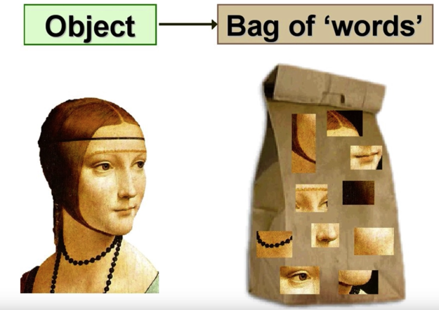
Object instance recognition
- Visual words
- Quantization, index, bags of words
Indexing Local Features
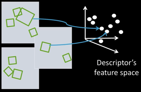
- Each patch/region has a descriptor, which is a point in some high-dimensional feature space (e.g., SIFT)
- When we see close points in feature space, we have similar descriptors, which indicates similar local content
- The problem: any given image easily can have millions of features to search

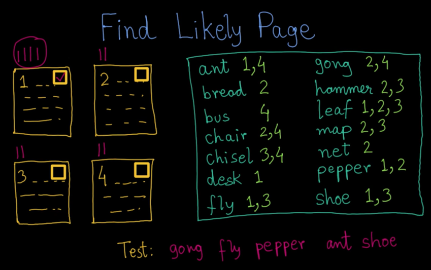
Inverted File Index
- With potentially thousands of features per image, and hundreds to millions of images to search, how to efficiently find those that are relevant to a new image?
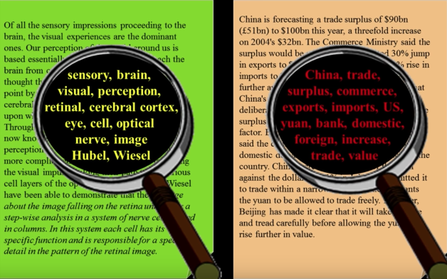
Indexing local features: inverted file index
- For text documents, and efficient way to find all pages on which a word occurs is to use an index...
- We want to find all images in which a feature occurs
- To use this idea, we'll need to map our features to "visual words"

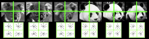
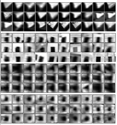
Visual words
Example: each group of patches belongs to the same visual word

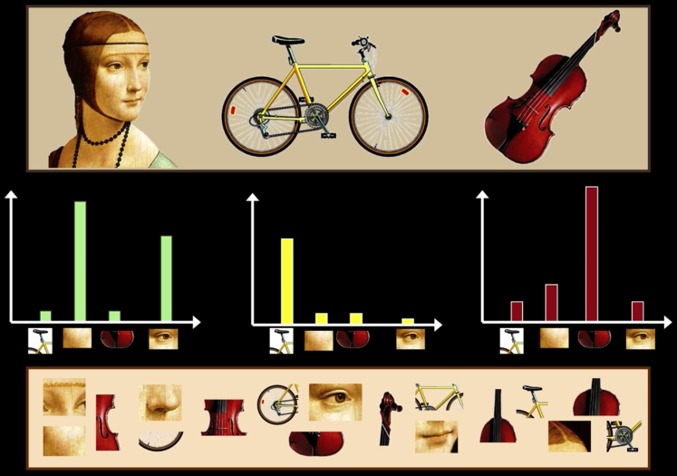
Comparing Bags of Words
- Rank by normalized scalar product between their (possibly weighted) occurrence counts -- nearest neighbor search for similar images.

$$sim(d_j,q) = \frac{<d_j,q>}{||d_j||||q||}$$
$$= \frac{\sum_{i=1}^Vd_j(i)*q(i)}{\sqrt{\sum_{i=1}^Vd_j(i)^2}*\sqrt{\sum_{i=1}^Vq(i)^2}}$$
Object Classification with Bag of Words
- Performance on Caltech 101 dataset with linear SVM on bag-of-word vectors:
"""
Object Classification with Bag of Words
Source: https://github.com/kushalvyas/Bag-of-Visual-Words-Python
Author: kushalvyas
"""
import cv2
import numpy as np
from glob import glob
from sklearn.cluster import KMeans
from sklearn.svm import SVC
from sklearn.preprocessing import StandardScaler
from matplotlib import pyplot as plt
## Helper Classes
class ImageHelpers:
def __init__(self):
self.sift_object = cv2.xfeatures2d.SIFT_create()
def gray(self, image):
gray = cv2.cvtColor(image, cv2.COLOR_BGR2GRAY)
return gray
def features(self, image):
keypoints, descriptors = self.sift_object.detectAndCompute(image, None)
return [keypoints, descriptors]
class BOVHelpers:
def __init__(self, n_clusters = 20):
self.n_clusters = n_clusters
self.kmeans_obj = KMeans(n_clusters = n_clusters)
self.kmeans_ret = None
self.descriptor_vstack = None
self.mega_histogram = None
self.clf = SVC()
def cluster(self):
"""
cluster using KMeans algorithm,
"""
self.kmeans_ret = self.kmeans_obj.fit_predict(self.descriptor_vstack)
def developVocabulary(self,n_images, descriptor_list, kmeans_ret = None):
"""
Each cluster denotes a particular visual word
Every image can be represeted as a combination of multiple
visual words. The best method is to generate a sparse histogram
that contains the frequency of occurence of each visual word
Thus the vocabulary comprises of a set of histograms of encompassing
all descriptions for all images
"""
self.mega_histogram = np.array([np.zeros(self.n_clusters) for i in range(n_images)])
old_count = 0
for i in range(n_images):
l = len(descriptor_list[i])
for j in range(l):
if kmeans_ret is None:
idx = self.kmeans_ret[old_count+j]
else:
idx = kmeans_ret[old_count+j]
self.mega_histogram[i][idx] += 1
old_count += l
print("Vocabulary Histogram Generated")
def standardize(self, std=None):
"""
standardize is required to normalize the distribution
wrt sample size and features. If not normalized, the classifier may become
biased due to steep variances.
"""
if std is None:
self.scale = StandardScaler().fit(self.mega_histogram)
self.mega_histogram = self.scale.transform(self.mega_histogram)
else:
print("STD not none. External STD supplied")
self.mega_histogram = std.transform(self.mega_histogram)
def formatND(self, l):
"""
restructures list into vstack array of shape
M samples x N features for sklearn
"""
vStack = np.array(l[0])
for remaining in l[1:]:
vStack = np.vstack((vStack, remaining))
self.descriptor_vstack = vStack.copy()
return vStack
def train(self, train_labels):
"""
uses sklearn.svm.SVC classifier (SVM)
"""
print ("Training SVM")
print (self.clf)
print ("Train labels", train_labels)
self.clf.fit(self.mega_histogram, train_labels)
print ("Training completed")
def predict(self, iplist):
predictions = self.clf.predict(iplist)
return predictions
def plotHist(self, vocabulary = None):
print("Plotting histogram")
if vocabulary is None:
vocabulary = self.mega_histogram
x_scalar = np.arange(self.n_clusters)
y_scalar = np.array([abs(np.sum(vocabulary[:,h], dtype=np.int32)) for h in range(self.n_clusters)])
print (y_scalar)
fig = plt.gcf()
fig.set_size_inches((20,10))
plt.bar(x_scalar, y_scalar)
plt.xlabel("Visual Word Index")
plt.ylabel("Frequency")
plt.title("Complete Vocabulary Generated")
plt.xticks(x_scalar + 0.4, x_scalar)
plt.show()
class FileHelpers:
def __init__(self):
pass
def getFiles(self, path):
"""
- returns a dictionary of all files
having key => value as objectname => image path
- returns total number of files.
"""
imlist = {}
count = 0
for each in glob(path + "*"):
word = each.split("/")[-1]
#print (" #### Reading image category ", word, " ##### ")
imlist[word] = []
for imagefile in glob(path+word+"/*"):
#print ("Reading file ", imagefile)
im = cv2.imread(imagefile, 0)
imlist[word].append(im)
count +=1
return [imlist, count]
## Bag of words Classes
from glob import glob
from matplotlib import pyplot as plt
class BOV:
def __init__(self, no_clusters):
self.no_clusters = no_clusters
self.train_path = None
self.test_path = None
self.im_helper = ImageHelpers()
self.bov_helper = BOVHelpers(no_clusters)
self.file_helper = FileHelpers()
self.images = None
self.trainImageCount = 0
self.train_labels = np.array([])
self.name_dict = {}
self.descriptor_list = []
def trainModel(self):
"""
This method contains the entire module
required for training the bag of visual words model
Use of helper functions will be extensive.
"""
# read file. prepare file lists.
self.images, self.trainImageCount = self.file_helper.getFiles(self.train_path)
# extract SIFT Features from each image
label_count = 0
for word, imlist in self.images.items():
self.name_dict[str(label_count)] = word
print("Computing Features for ", word)
for im in imlist:
# cv2.imshow("im", im)
# cv2.waitKey()
self.train_labels = np.append(self.train_labels, label_count)
kp, des = self.im_helper.features(im)
self.descriptor_list.append(des)
label_count += 1
# perform clustering
bov_descriptor_stack = self.bov_helper.formatND(self.descriptor_list)
self.bov_helper.cluster()
self.bov_helper.developVocabulary(n_images = self.trainImageCount, descriptor_list=self.descriptor_list)
# show vocabulary trained
self.bov_helper.plotHist()
self.bov_helper.standardize()
self.bov_helper.train(self.train_labels)
def recognize(self,test_img, test_image_path=None):
"""
This method recognizes a single image
It can be utilized individually as well.
"""
kp, des = self.im_helper.features(test_img)
# print kp
#print(des.shape)
# generate vocab for test image
vocab = np.array( [[ 0 for i in range(self.no_clusters)]])
# locate nearest clusters for each of
# the visual word (feature) present in the image
# test_ret =<> return of kmeans nearest clusters for N features
test_ret = self.bov_helper.kmeans_obj.predict(des)
# print test_ret
# print vocab
for each in test_ret:
vocab[0][each] += 1
#print(vocab)
# Scale the features
vocab = self.bov_helper.scale.transform(vocab)
# predict the class of the image
lb = self.bov_helper.clf.predict(vocab)
# print "Image belongs to class : ", self.name_dict[str(int(lb[0]))]
return lb
def testModel(self):
"""
This method is to test the trained classifier
read all images from testing path
use BOVHelpers.predict() function to obtain classes of each image
"""
self.testImages, self.testImageCount = self.file_helper.getFiles(self.test_path)
predictions = []
for word, imlist in self.testImages.items():
#print("processing " ,word)
for im in imlist:
# print imlist[0].shape, imlist[1].shape
#print(im.shape)
cl = self.recognize(im)
#print(cl)
predictions.append({
'image':im,
'class':cl,
'object_name':self.name_dict[str(int(cl[0]))]
})
#print(predictions)
for each in predictions:
# cv2.imshow(each['object_name'], each['image'])
# cv2.waitKey()
# cv2.destroyWindow(each['object_name'])
#
plt.imshow(cv2.cvtColor(each['image'], cv2.COLOR_GRAY2RGB))
plt.title(each['object_name'])
plt.show()
def print_vars(self):
pass
bov = BOV(no_clusters=100)
# set training paths
bov.train_path = "bagofwords/images/train/"
# set testing paths
bov.test_path = "bagofwords/images/test/"
# train the model
bov.trainModel()
# test model
bov.testModel()


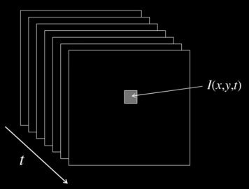
Video
A video is a sequence of frames captured over time
- Now our image data is a function of space $\color{blue}{(x,y)}$ and time $\color{blue}{(t)}$
Processing video: Object detection
If the goial of "activity recognition" is to recognize the activity of objects...
... you (may) have to fine the objects...
Background subtraction

- Needs static camera - still hard!
- Widely used:
- Traffic monitoring (counting vehicles, detecting & tracking vehicles, pedestrians)
- Human action recognition (run, walk, jump, squat)
- Human-computer interaction
- Object tracking
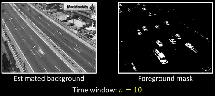
Simple approach
- Estimate background for time $\color{blue}{t}$
- Subtract estimated background from current input frame
- Apply a threshold to the absolute difference to get the forground mask

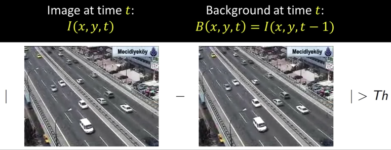
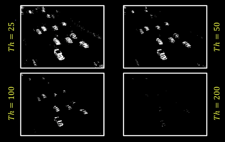
Frame differencing
Background is estimated to be the previous frame
$$\color{blue}{B(x,y,t) = I(x,y,t-1)}$$
Background subtraction then becomes:
$$\color{blue}{|I(x,y,t) - I(x,y,t-1)|> Th}$$
Mean Filtering
In this case, background is the mean of the previous $\color{blue}{n}$ frames:
$$\color{blue}{B(x,y,t) = \frac{1}{n}\sum_{i=1}^n I(x,y,t-1)}$$
Therefore, foreground mask is computed as:
$$\color{blue}{\left |I(x,y,t)- \frac{1}{n}\sum_{i=1}^n I(x,y,t-1)\right | > Th}$$

import os, numpy, PIL
from PIL import Image
import numpy as np
# Access all PNG files in directory
allfiles=os.listdir("imgs/bkgs/")
imlist=["imgs/bkgs/"+filename for filename in allfiles if filename[-4:] in [".png",".PNG"]]
imlist = sorted(imlist)
# Assuming all images are the same size, get dimensions of first image
w,h=Image.open(imlist[0]).size
N=len(imlist)
# Create a numpy array of floats to store the average (assume RGB images)
arr=numpy.ones((h,w,3),numpy.float)*255
# Build up average pixel intensities, casting each image as an array of floats
imgs = []
for im in imlist:
imgs.append(Image.open(im))
imarr=numpy.array(imgs[-1],dtype=numpy.float)[:,:,:3]
arr=arr+imarr/N
# Round values in array and cast as 8-bit integer
arr=numpy.array(numpy.round(arr),dtype=numpy.uint8)
# Generate, save and preview final image
mean_image=Image.fromarray(arr,mode="RGB")
import matplotlib.pyplot as plt
fig, ax = plt.subplots(nrows=len(imgs)+1)
fig.set_size_inches((20,30))
for i,img in enumerate(imgs):
ax[i].imshow(imgs[i])
ax[i].set_title("Frame: %d" % i)
ax[i].xaxis.set_major_locator(plt.NullLocator())
ax[i].yaxis.set_major_locator(plt.NullLocator())
ax[-1].imshow(mean_image)
ax[-1].set_title("Background Mean Image")
ax[-1].yaxis.set_major_locator(plt.NullLocator())
ax[-1].xaxis.set_major_locator(plt.NullLocator())
plt.show()

Median Filtering
Assuming that the background is more likely to appear in a scene, we can use the median of previous $\color{blue}{n}$ frames as the background model:
$$\color{blue}{B(x,y,t) = median\{I(x,y,t-i)\}}$$
Therefore, foreground mask is computed as:
$$\color{blue}{|I(x,y,t-i)-median\{I(x,y,t-i)\}|> Th}$$
$$\text{where }\color{blue}{i \in \{1,...n\}}$$
import os, numpy, PIL
from PIL import Image
# Access all PNG files in directory
allfiles=os.listdir("imgs/bkgs/")
imlist=["imgs/bkgs/"+filename for filename in allfiles if filename[-4:] in [".png",".PNG"]]
imlist = sorted(imlist)
# Assuming all images are the same size, get dimensions of first image
w,h=Image.open(imlist[0]).size
N=len(imlist)
imgsarr = []
imgs = []
for im in imlist:
imgs.append(Image.open(im))
imgsarr.append(np.asarray(imgs[-1])[:,:,:3])
# Convert images to 4d ndarray, size(n, nrows, ncols, 3)
imgsarr = np.asarray(imgsarr)
# Take the median over the first dim
med = np.median(imgsarr, axis=0)
arr=numpy.array(numpy.round(med),dtype=numpy.uint8)
median_image=Image.fromarray(arr,mode="RGB")
import matplotlib.pyplot as plt
fig, ax = plt.subplots(nrows=len(imgs)+1)
fig.set_size_inches((20,30))
for i,img in enumerate(imgs):
ax[i].imshow(imgsarr[i])
ax[i].set_title("Frame: %d" % i)
ax[i].xaxis.set_major_locator(plt.NullLocator())
ax[i].yaxis.set_major_locator(plt.NullLocator())
ax[-1].imshow(median_image)
ax[-1].set_title("Background Median Image")
ax[-1].yaxis.set_major_locator(plt.NullLocator())
ax[-1].xaxis.set_major_locator(plt.NullLocator())
plt.show()

import cv2
plt.imshow(imgs[0])
fig, ax = plt.subplots(nrows=1,ncols=2)
fig.set_size_inches((20,20))
meanimg_arr = np.asarray(mean_image)
cv2.rectangle(meanimg_arr,(380,150),(600,280),(255,0,0),3)
ax[0].imshow(meanimg_arr)
ax[0].set_title("Background Mean Image")
medimg_arr = np.asarray(median_image)
cv2.rectangle(medimg_arr,(380,150),(600,280),(255,0,0),3)
ax[1].imshow(medimg_arr)
ax[1].set_title("Background Median Image")
plt.show()


from PIL import ImageChops
def trim(im):
bg = Image.new(im.mode, im.size, im.getpixel((0,0)))
diff = ImageChops.difference(im, bg)
diff = ImageChops.add(diff, diff, 2.0, -100)
bbox = diff.getbbox()
if bbox:
return im.crop(bbox)
img = trim(median_image)
img.save("imgs/background.jpg")
## Using OpenCV
## Run this outside the notebook to exit gracefully
# import numpy as np
# import cv2
# cap = cv2.VideoCapture('imgs/people-walking.mp4')
# fgbg = cv2.createBackgroundSubtractorMOG2()
# while(1):
# ret, frame = cap.read()
# fgmask = fgbg.apply(frame)
# cv2.imshow('fgmask',frame)
# cv2.imshow('frame',fgmask)
# k = cv2.waitKey(30) & 0xff
# if k == 27:
# break
# cap.release()
# cv2.destroyAllWindows()
Pros and Cons
Advantages:
- Extremely easy to implement and use!
- All pretty fast
- Corresponding background models need not be constant, they change over time
Disadvantages:
- Accuracy of frame differencing depends on object speed and frame rate
- Median background mode - relatively high memory requirements
- Setting global threshold $\color{blue}{Th}$...
When will this basic approach fail?

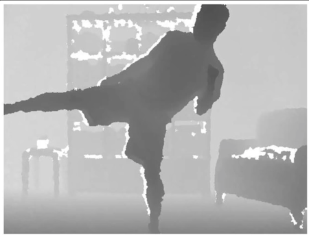


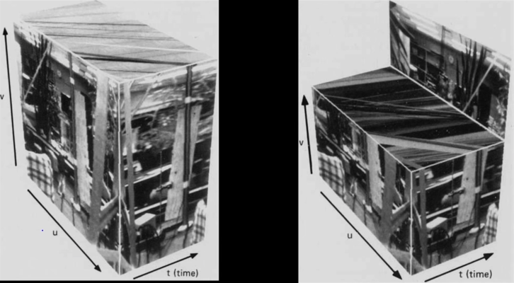


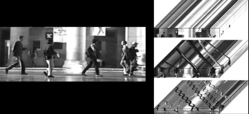
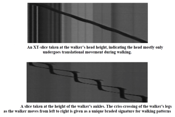

Human activity in video
No universal terminology, but approximately:
Event: A single instant in time detection
Actions or Movements: Atomic motion patterns
- Often gesture-like
- Single clear-cut trajectory
- Single nameable behavior (e.g., sit, wave arms)
Activity: Series or composition of actions
- E.g., interactions between people
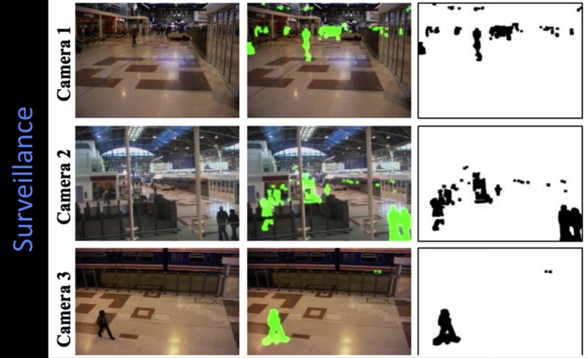
Human Activity in Video
Model-based action recognition
- Use human body tracking and pose estimation techniques, relate to action descriptions (or learn)
- Major challenge: training data from different context than testing
Model-based activity recognition
- Given some lower level detection of actions (or events) recognize the activity by comparing to some structural representation of the activity
- Needs to handle uncertainty
- Major challenge: Accurate tracks in spite of occlusion, ambiguity, low resolution
- Recently activity as motion, space-time, appearance patterns
- Describe overall patterns, but no explicit body tracking
- Typically learn classifier
- Also recently: Activity-recognition from a static image
- Imagine a picture of a person holding a flute
- What are they doing?
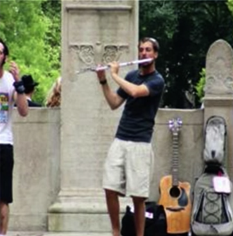

Motion History Images
Even "impoverished" motion data can evoke a strong percept


Motion Energy Images
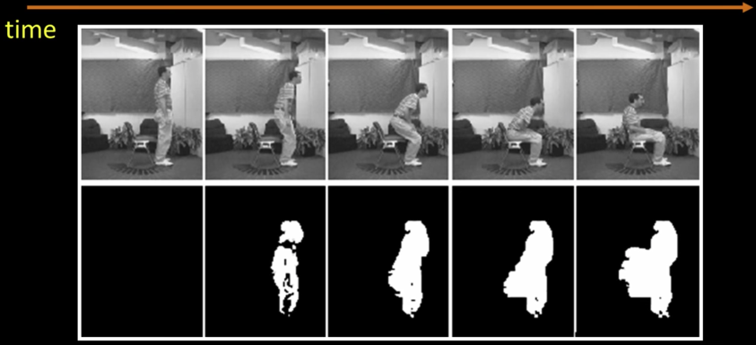
MHIs are a different function of temporal volume
- Pixel operator is replacement decay:

if moving:
$\color{blue}{I_\tau(x,y,t) = \tau}$
otherwise:
$\color{blue}{I_\tau(x,y,t) = max(I_\tau(x,y,t-1)-1,0)}$
Trivial to construct $\color{blue}{I_{\tau-k}(x,y,t)}$ from $\color{blue}{I_{\tau}(x,y,t)}$ - so we can process multiple time window lengths without additional image analysis
MEI is thresholded MHI
## Calculating Motion Energy Image
import numpy as np
import cv2
def imread(filename):
img = cv2.imread(filename)
img = cv2.cvtColor(img, cv2.COLOR_BGR2RGB)
return img
cap = cv2.VideoCapture('imgs/people-walking.mp4')
nFrames = int(cap.get(cv2.CAP_PROP_FRAME_COUNT))
back_frame = gray(imread('imgs/background.jpg'))
x,y = back_frame.shape
mei = np.zeros((x,y));
# get the motion energy image with threshold of 40
# This will take sometime
for i in range(nFrames):
print("Processing frame %d/%d" % (i,nFrames))
ret, frame = cap.read()
grayframe = gray(frame)
foreground1 = abs(back_frame.astype(np.float) - grayframe.astype(np.float))
for i in range(x):
for j in range(y):
if foreground1[i,j] < 40:
mei[i,j] = mei[i,j]+0
else:
mei[i,j] = mei[i,j]+255
## to not modify the previous step calculation
mei2 = mei.copy().astype(np.uint8)
imshow(mei2)

from scipy.signal import medfilt2d as medfilt2
fg_filt = medfilt2(mei2, [5,5]);
imshow(fg_filt);

## Calculating Motion History Image
cap = cv2.VideoCapture('imgs/people-walking.mp4')
nFrames = int(cap.get(cv2.CAP_PROP_FRAME_COUNT))
back_frame = gray(imread('imgs/background.jpg'))
x,y = back_frame.shape
mhi = np.zeros((x,y));
for i in range(nFrames):
print("Processing frame %d/%d" % (i,nFrames))
ret, frame = cap.read()
grayframe = gray(frame)
foreground1 = abs(back_frame.astype(np.float) - grayframe.astype(np.float))
foreground1 = foreground1.astype(np.uint8)
for i in range(x):
for j in range(y):
if foreground1[i,j] < 50:
mhi[i,j] = mhi[i,j] - 0.15
else:
mhi[i,j] = mhi[i,j] = 255
mhi2 = mhi.copy().astype(np.uint8)
imshow(mhi2)

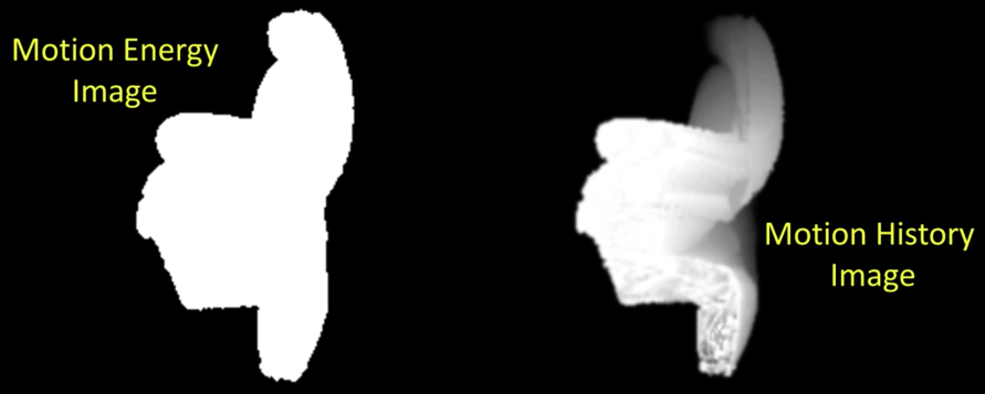


Image Moments
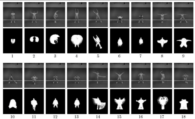
How to recognize these images?
- In 1999, old style computer vision:
- Compute some summarization statistics of the pattern
- Construct generative model
- Recognize based upon those statistics
Image moments:
Moments summarize a shape given image $\color{blue}{I(x,y)}$
$$\color{blue}{M_{ij} = \sum_x\sum_yx^iy^jI(x,y)}$$
Central moments are translation invariant:
$$\color{blue}{\mu_{pq} = \sum_x\sum_y(x-\bar{x})^p(y-\bar{y})^qI(x,y)}$$
$$\color{blue}{\bar{x} = \frac{M_{10}}{M_{00}}}$$
$$\color{blue}{\bar{y} = \frac{M_{01}}{M_{00}}}$$
Hu moments
- Translation and rotation and scale invariant
- We chose 7 moments
- Apply to Motion History Image for global space-time "shape" descriptor
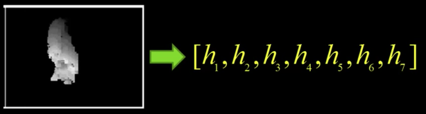
$$\color{blue}{h_1 = \mu_{20}+\mu_{02}}$$
$$\color{blue}{h_2 = (\mu_{20}-\mu_{02})^2+4\mu^2_{11}}$$
$$\color{blue}{h_3 = (\mu_{30}-3\mu_{12})^2+(3\mu_{21}-\mu_{03})^2}$$
$$\color{blue}{h_4 = (\mu_{30}+\mu_{12})^2+(\mu_{21}-\mu_{03})^2}$$
$$\color{blue}{h_5 = (\mu_{30}-3\mu_{12})(\mu_{30}+\mu_{12})[(\mu_{30}+\mu_{12})^2-3(\mu_{21}+\mu_{03})^2]+(3\mu_{21}-\mu_{03})(\mu_{21}+\mu_{03})[3(\mu_{30}+\mu_{12})^2-(\mu_{21}+\mu_{03})^2]}$$
$$\color{blue}{h_6 = (\mu_{20}-\mu_{02})[(\mu_{30}+\mu_{12})^2-(\mu_{21}+\mu_{03})^2]+4\mu_{11}(\mu_{30}+\mu_{12})(\mu_{21}+\mu_{03})}$$
$$\color{blue}{h_7 = (3\mu_{21}-\mu_{03})(\mu_{30}+\mu_{12})[(\mu_{30}+\mu_{12})^2-3(\mu_{21}+\mu_{03})^2]-(\mu_{30}-3\mu_{12})(\mu_{21}+\mu_{03})[3(\mu_{30}+\mu_{12})^2-(\mu_{21}+\mu_{03})^2]}$$
## Source: https://www.learnopencv.com/shape-matching-using-hu-moments-c-python/
import glob
import cv2
from math import copysign, log10
showLogTransformedHuMoments = True
allfiles=os.listdir("humoments/imgs/")
imlist=["humoments/imgs/"+filename for filename in allfiles if filename[-4:] in [".png",".PNG"]]
for i in range(len(imlist)):
# Obtain filename from command line argument
filename = imlist[i]
# Read image
im = cv2.imread(filename,cv2.IMREAD_GRAYSCALE)
# Threshold image
_,im = cv2.threshold(im, 128, 255, cv2.THRESH_BINARY)
# Calculate Moments
moment = cv2.moments(im)
# Calculate Hu Moments
huMoments = cv2.HuMoments(moment)
# Print Hu Moments
print("{}: ".format(filename),end='')
for i in range(0,7):
if showLogTransformedHuMoments:
# Log transform Hu Moments to make
# squash the range
print("{:.5f}".format(-1*copysign(1.0,huMoments[i])*log10(abs(huMoments[i]))),end=' ')
else:
# Hu Moments without log transform
print("{:.5f}".format(huMoments[i]),end=' ')
print()
Build a classifier
Remember Generative vs Discriminative
Generative - builds model of each class; compare all
Discriminative - builds model of the boundary between classes
How would you build decent generative models of each class of action?
- Use a Gaussian in Hu-moment feature space
- Compare likelihoods: $\color{blue}{p(data|\text{model of action i)}}$
- If have priors, use them by Bayes rule
$$\color{blue}{p(model_i|data) \propto p(data|model_i)p(model)}$$
- Otherwise just use likelihood. Or oven NN
## Using hu to find similarity. The least the value, the more similar two images are
import cv2
im1 = cv2.imread("humoments/imgs/S0.png",cv2.IMREAD_GRAYSCALE)
im2 = cv2.imread("humoments/imgs/K0.png",cv2.IMREAD_GRAYSCALE)
im3 = cv2.imread("humoments/imgs/S4.png",cv2.IMREAD_GRAYSCALE)
imshow(im1)
imshow(im2)
imshow(im3)
m1 = cv2.matchShapes(im1,im1,cv2.CONTOURS_MATCH_I2,0)
m2 = cv2.matchShapes(im1,im2,cv2.CONTOURS_MATCH_I2,0)
m3 = cv2.matchShapes(im1,im3,cv2.CONTOURS_MATCH_I2,0)
print("Shape Distances Between \n-------------------------")
print("S0.png and S0.png : {}".format(m1))
print("S0.png and K0.png : {}".format(m2))
print("S0.png and S4.png : {}".format(m3))


KidsRoom
Recognizing temporal templates
- Linear time scaling
- Compute range of $\tau$ using the min and max of training data
- Simple recursive fomulation so very fast
- Filter implementation obvious so biologically "relevant"
- Best reference is PAMI 2001, Bobick and Davis
Virtual PAT (Personal Aerobics Trainer)
- Use MHI recognition
- Portable IR background subtraction system (CAPTECH '98)

The KidsRoom
- First teach the kids, then observe
- Temporal templates "plus" (but in paper)
- Monsters always do something, but only speak it when sure
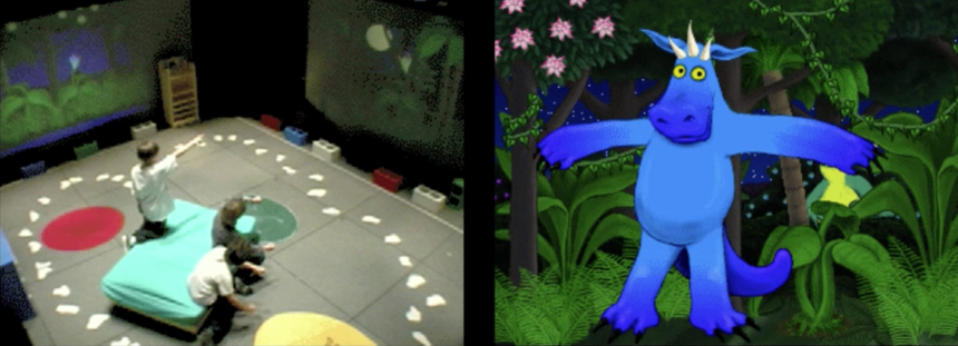
Outline
- Time Series
- Markov Models
- Hidden Markov Models
- 3 computational problems of HMMs
- Applying HMMs in vision- Gesture
Questions One Could Ask
Audio Spectrum

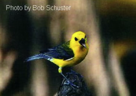

Questions One Could Ask
- What bird is this? > Time series classification
- How will the song continue? > Time series prediction
- Is this bird sick? > Outlier detection
- What phases does this song have? > Time series segmentation
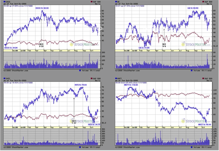
- Will this stock go up or down? > Time series prediction
- What type stock is this (eg, risky)? > Time series classification
- Is the behavior abnormal? > Outlier detection
Music Analysis

- Is this Beethoven or Bach? > Time series classification
- Can we compose more of that? > Time series prediction/generation
- Can we segment the piece into themes? > Time series segmentation

Markov Models
Weather: A Markov Model (maybe?)
- $1^{st}$ Order Markovian: Probability of moving to a given state depends only on the current state

Ingredients of a Markov Model
States: $\color{blue}{\{S_1,S_2,...,S_N\}}$
State transition probabilities: $\color{blue}{a_{ij} = P(q_{t+1} = S_i|q_t = S_j)}$
Intial state distribution: $\color{blue}{\pi_i = P[q_1 = S_i]}$
For the example in Fig(70):
States: $\color{#b841f4}{\{S_{sunny},S_{rainy},S_{snowy}\}}$
State transition probabilities: $$\color{#b841f4}{A = \begin{bmatrix}0.8&0.15&0.05\\0.38&0.6&0.02\\0.75&0.05&0.2\end{bmatrix}}$$
Intial state distribution: $\color{#b841f4}{\pi = (0.7,0.25,0.05)}$
Probability of a time series
- Given:

- What is the probability of this series?
$$\color{blue}{P(S_{sunny})\cdot P(S_{rainy}|S_{sunny})\cdot P(S_{rainy}|S_{rainy})\cdot P(S_{rainy}|S_{rainy})\cdot P(S_{snowy}|S_{rainy})\cdot P(S_{snowy}|S_{snowy}) }$$
$$\color{blue}{=0.7\cdot 0.15\cdot 0.6\cdot 0.6\cdot 0.02\cdot 0.2 = 0.0001512}$$
import numpy as np
A = np.array([[0.8,0.15,0.05],[0.38,0.6,0.02],[0.75,0.05,0.2]])
psunny = 0.7
prainy = 0.25
psnowy = 0.05
pi = [psunny,prainy,psnowy]
#𝑃(𝑆𝑠𝑢𝑛𝑛𝑦)⋅𝑃(𝑆𝑟𝑎𝑖𝑛𝑦|𝑆𝑠𝑢𝑛𝑛𝑦)⋅𝑃(𝑆𝑟𝑎𝑖𝑛𝑦|𝑆𝑟𝑎𝑖𝑛𝑦)⋅𝑃(𝑆𝑟𝑎𝑖𝑛𝑦|𝑆𝑟𝑎𝑖𝑛𝑦)⋅𝑃(𝑆𝑠𝑛𝑜𝑤𝑦|𝑆𝑟𝑎𝑖𝑛𝑦)⋅𝑃(𝑆𝑠𝑛𝑜𝑤𝑦|𝑆𝑠𝑛𝑜𝑤𝑦
psunny*A[0,1]*A[1,1]*A[1,1]*A[1,2]*A[2,2]
Hidden Markov Models
Observables:
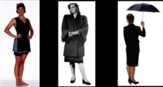
Emission probabilities
$$\color{blue}{b_j(k) = P(o_t = k) | q_t = S_i}$$
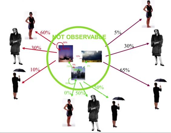
- Given:
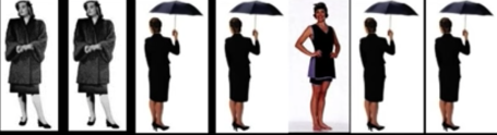
- What is the probability of this series?
$$P(O) = P(O_{coat},O_{coat},O_{umbrella},...,O_{umbrella})$$
$$= \sum_{all\, Q} P(O|Q)P(Q) = \sum_{q1,...,q_7}P(O|q_1,...,q_7)P(q_1,...,q_7)$$
$$= \color{#00abab}{(0.3^2\cdot0.1^4\cdot0.6)}\color{blue}{\cdot(0.7\cdot0.8^6)}+...$$
$\color{#b841f4}{A = \begin{bmatrix}0.8&0.15&0.05\\0.38&0.6&0.02\\0.75&0.05&0.2\end{bmatrix}}$ $\color{#b841f4}{\{S_{sunny},S_{rainy},S_{snowy}\}}$ $\color{#00abab}{B = \begin{bmatrix}0.6&0.3&0.1\\0.05&0.3&0.65\\0&0.5&0.5\end{bmatrix}}$
Specification of an HMM
- N - number of states
- $S = \{S_1,S_2,...,S_N\}$ - set of states
- $Q = \{q_1,q_2,...,q_T\}$ - sequence of states
Specification of an HMM: $\lambda = (A,B,\pi)$
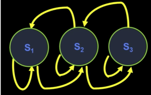
A- the state transition probability matrix
$$\color{blue}{a_{ij} = P(q_{t+1} = j | q_t = i)}$$
B- observation probability distribution
- Discrete: $\color{blue}{b_j(k) = P(o_t = k | q_t = j) 1\le k \le M}$
- Continuous: $\color{blue}{b_j(x) = P(o_t = x | q_t = j)}$
$\pi$ - the initial state distribution
$$\color{blue}{\pi(j) = P(q_1 = j)}$$
What does this have to do with Vision
Given some sequence of observations, what "model" generated those?
Using the previous example: given some observation sequence of clothing:
Is this Philadelphia, Boston or Newark?
Notice that if Boston vs Arizona would not need the sequence?
The 3 Great Problems in HMM Modeling
- Evaluation $\color{blue}{P(O|\lambda)}$: Given the model $\color{blue}{\lambda = (A,B,\pi)}$, what is the probability of occurrence of a particular observation sequence
$$\color{blue}{O = \{o_1,...,o_T\}}$$
- Classification/recognition problem: I have a trained model for each of a set of classes, which one would most likely generate what I saw
Decoding: Optimal state sequence to produce an observation sequence $\color{blue}{o_1,...,o_T}$
Useful in recognition problems - helps give meaning to states -
Learning: Detemine model $\color{blue}{\lambda}$, given a training set of observations
Find $\color{blue}{\lambda}$, such that $\color{blue}{P(O|\lambda)}$ is maximal
Naive Solution
Problem $1 P(O|\lambda)$: Naive solution
Assume
- We know state sequence $\color{blue}{Q = (q_1,...q_T)}$
- Independent observations:
$$\color{blue}{P(O|q,\lambda) = \prod^T_{i=1} P(o_t|q_t,\lambda) = b_{q1}(o_1)b_{q2}(o_2)...b_{qT}(O_T)}$$
- But we know the probability of any given sequence of states
$$\color{blue}{P(q|\lambda) = \pi_{q1}a_{q1q1}a_{q2q3}....a_{q(T-1)qT}}$$
- Given the previous two calculations
- We get: $\color{blue}{P(O|\lambda) = \sum_q P(O|q,\pi)P(q|\lambda)}$
But this is summed over all paths. There are $N^T$ states paths, each 'coasting' O(T) calculations, leading to $O(TN^T)$ time complexity
Efficient solution
Define auxiliary forward variables $\alpha$
$$\color{blue}{\alpha_t(i) = P(o_1,...,o_t,q_t = i|\lambda)}$$
$a_t(i)$ is the probability of observing a partial sequence of observables $o_1,...,o_t$ AND at time $t$, state $q_t=i$
Forward Recursive algorithm:
- Initialise: $\color{blue}{\alpha_1(i) = \pi_i b_i(o_1)}$
- Each time step: $\color{blue}{\alpha_{t+1}(j) = \left [\sim_{i=1}^N \alpha_t(i)a_{ij}\right ]b_j(o_{t+1})}$ (Can reach j from any preceding state)
- Conclude: $\color{blue}{P(O|\lambda) = \sum_{i=1}^N\alpha_T(i)}$ (Probability of the entire observation sequence is just sum of observations and ending up in state i, for all i)
- Complexity: $\color{red}{O(N^2T)}$
## THIS CODE IS TAKEN FROM https://www.digitalvidya.com/blog/inroduction-to-hidden-markov-models-using-python/
## DISCRIPTION OF THE PROBLEM TARGETED IN THIS CODE IS IN THE LINK
import numpy as np
import pandas as pd
import networkx.drawing.nx_pydot as gl
import networkx as nx
import matplotlib.pyplot as plt
from pprint import pprint
##matplotlib inline
# create state space and initial state probabilities
states = ['O1', 'O2', 'O3']
pi = [0.25, 0.4, 0.35]
state_space = pd.Series(pi, index=states, name='states')
print(state_space)
print(state_space.sum())
# create transition matrix
# equals transition probability matrix of changing states given a state
# matrix is size (M x M) where M is number of states
q_df = pd.DataFrame(columns=states, index=states)
q_df.loc[states[0]] = [0.4, 0.2, 0.4]
q_df.loc[states[1]] = [0.45, 0.45, 0.1]
q_df.loc[states[2]] = [0.45, 0.25, .3]
print(q_df)
q = q_df.values
print('\n')
print(q, q.shape)
print('\n')
print(q_df.sum(axis=1))
from pprint import pprint
# create a function that maps transition probability dataframe
# to markov edges and weights
def _get_markov_edges(Q):
edges = {}
for col in Q.columns:
for idx in Q.index:
edges[(idx,col)] = Q.loc[idx,col]
return edges
edges_wts = _get_markov_edges(q_df)
pprint(edges_wts)
# create graph object
G = nx.MultiDiGraph()
# nodes correspond to states
G.add_nodes_from(states)
print('Nodes:\n')
print(G.nodes())
print('\n')
# edges represent transition probabilities
for k, v in edges_wts.items():
tmp_origin, tmp_destination = k[0], k[1]
G.add_edge(tmp_origin, tmp_destination, weight=v, label=v)
print('Edges:')
pprint(G.edges(data=True))
pos = nx.drawing.nx_pydot.graphviz_layout(G, prog='dot')
nx.draw_networkx(G, pos)
# create edge labels for jupyter plot but is not necessary
edge_labels = {(n1,n2):d['label'] for n1,n2,d in G.edges(data=True)}
nx.draw_networkx_edge_labels(G , pos, edge_labels=edge_labels)
nx.drawing.nx_pydot.write_dot(G, 'markov.dot')
plt.show()

# create state space and initial state probabilities
hidden_states = ['S1', 'S2']
pi = [0.5, 0.5]
print('\n')
state_space = pd.Series(pi, index=hidden_states, name='states')
print(state_space)
print('\n')
print(state_space.sum())
# create hidden transition matrix
# a or alpha
# = transition probability matrix of changing states given a state
# matrix is size (M x M) where M is number of states
a_df = pd.DataFrame(columns=hidden_states, index=hidden_states)
a_df.loc[hidden_states[0]] = [0.7, 0.3]
a_df.loc[hidden_states[1]] = [0.4, 0.6]
print(a_df)
a = a_df.values
print('\n')
print(a)
print(a.shape)
print('\n')
print(a_df.sum(axis=1))
# create matrix of observation (emission) probabilities
# b or beta = observation probabilities given state
# matrix is size (M x O) where M is number of states
# and O is number of different possible observations
observable_states = states
b_df = pd.DataFrame(columns=observable_states, index=hidden_states)
b_df.loc[hidden_states[0]] = [0.2, 0.6, 0.2]
b_df.loc[hidden_states[1]] = [0.4, 0.1, 0.5]
print(b_df)
b = b_df.values
print('\n')
print(b)
print(b.shape)
print('\n')
print(b_df.sum(axis=1))
# create graph edges and weights
hide_edges_wts = _get_markov_edges(a_df)
pprint(hide_edges_wts)
emit_edges_wts = _get_markov_edges(b_df)
pprint(emit_edges_wts)
# create graph object
G = nx.MultiDiGraph()
# nodes correspond to states
G.add_nodes_from(hidden_states)
print('Nodes:\n')
print(G.nodes())
print('\n')
# edges represent hidden probabilities
for k, v in hide_edges_wts.items():
tmp_origin, tmp_destination = k[0], k[1]
G.add_edge(tmp_origin, tmp_destination, weight=v, label=v)
# edges represent emission probabilities
for k, v in emit_edges_wts.items():
tmp_origin, tmp_destination = k[0], k[1]
G.add_edge(tmp_origin, tmp_destination, weight=v, label=v)
print('Edges:')
pprint(G.edges(data=True))
pos = nx.drawing.nx_pydot.graphviz_layout(G, prog='neato')
nx.draw_networkx(G, pos)
plt.show()
# create edge labels
emit_edge_labels = {(n1,n2):d['label'] for n1,n2,d in G.edges(data=True)}
nx.draw_networkx_edge_labels(G , pos, edge_labels=emit_edge_labels)
plt.show()
nx.drawing.nx_pydot.write_dot(G, 'hidden_markov.dot')


# observation sequence of dog's behaviors
# observations are encoded numerically
obs_map = {'O1':0, 'O2':1, 'O3':2}
obs = np.array([1,1,2,1,0,1,2,1,0,2,2,0,1,0,1])
inv_obs_map = dict((v,k) for k, v in obs_map.items())
obs_seq = [inv_obs_map[v] for v in list(obs)]
print( pd.DataFrame(np.column_stack([obs, obs_seq]),
columns=['Obs_code', 'Obs_seq']) )
"""
Viterbi Algorithm
This algorithm finds the maximum probability of any
path to arrive at the state, i , at time t that also
has the correct observations for the sequence up to
time t.
"""
def viterbi(pi,a,b,obs):
nStates = np.shape(b)[0]
T = np.shape(obs)[0]
path = np.zeros(T)
delta = np.zeros((nStates,T))
phi = np.zeros((nStates,T))
delta[:,0] = pi * b[:,obs[0]]
phi[:,0] = 0
for t in range(1,T):
for s in range(nStates):
delta[s,t] = np.max(delta[:,t-1]*a[:,s])*b[s,obs[t]]
phi[s,t] = np.argmax(delta[:,t-1]*a[:,s])
path[T-1] = np.argmax(delta[:,T-1])
for t in range(T-2,-1,-1):
#path[t] = phi[int(path[t+1]): int(t+1) , int(t+1)]
path[t] = phi[int(path[t+1]) , int(t+1)]
return path,delta, phi
path, delta, phi = viterbi(pi, a, b, obs)
print('\n')
print('single best state path: ', path)
print('delta:\n', delta)
print('phi:\n', phi)
state_map = {0:'S1', 1:'S2'}
state_path = [state_map[v] for v in path]
result = (pd.DataFrame()
.assign(Observation=obs_seq)
.assign(Best_Path=state_path))
print(result)
Rest of HMMs in Words
The forward recursive algorithm could compute the likelihood of being in a state i at time t and having observed the sequence from the start until t, given HMM $\lambda$
A backword recursive algorithm could compute the likelihood of being in a state i at time t and observing the remainder of the observed sequence, given HMM $\lambda$
Hmmmmmm
If we know HMM $\lambda$ then with the forward and backward algorithm we can get an Estimate of the distribution over which state the system is in at ttime t
With those distributions and having actually observed output data, I can determine the emission probabilities $b_j(k)$ that would Maximize the probability of the sequence
Given distribution about state can also determine the transition probabilities $a_{ij}$ to Maximize probability
With the new $a_{ij}$ and $b_j(k)$ I can get a new estimate of the state distributions at all time (Go to 1)
HMMs: General
- HMMs: Generative probabilistic models of time series (with hidden state)
- Forward-Backward: Algorithm for computing probabilities over hidden states
- Given the forward-backward algorithms you can also train the models.
- Best know methods in speech, computer vision, robotics, though for really big data CRFs winning
Some Thoughts About Gesture
There is a conference on Face and Gesture Recognition so obviously Gesture recognition is an important problem
Prototype scenario:
- Subject does several examples of "each gesture"
- System "learns" (or is trained) to have some sort of model for each
- At run time compare input to known models and pick one
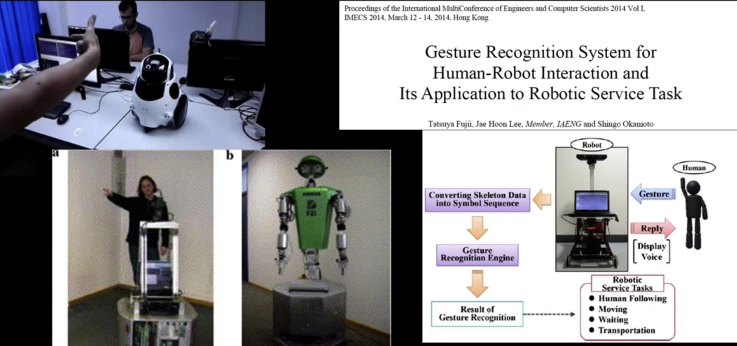
Generic Gesture Recognition
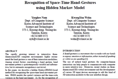

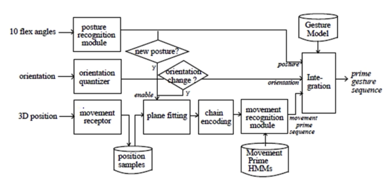
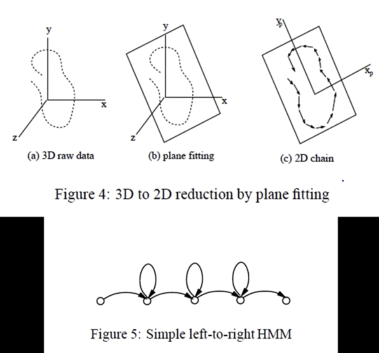
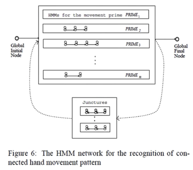
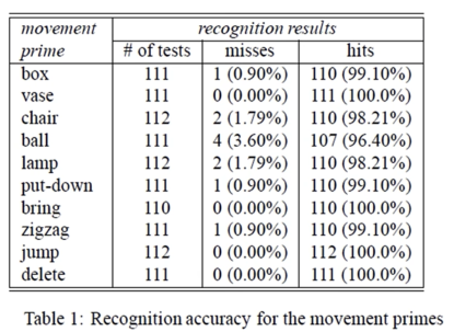
## Implementation of Gesture Recognition using HMM
## can be found in
## https://github.com/RajatBhageria/Gesture-Recognition-Using-Hidden-Markov-Models
# import numpy as np
# import glob
# import pickle
# import math
# from scipy.misc import logsumexp
# import sys
# sys.path.append("./Gesture-Recognition-Using-Hidden-Markov-Models/")
# Only = 1
# def predictTestGesture(folder = 'Gesture-Recognition-Using-Hidden-Markov-Models/train_data/*.txt'):
# # import all the IMU data
# file_list = glob.glob(folder)
# allData = np.empty((0, 5))
# kmfile = open('Gesture-Recognition-Using-Hidden-Markov-Models/kmeans_model.pickle', 'rb')
# u = pickle._Unpickler(kmfile)
# u.encoding = 'latin1'
# KMeansModel = u.load()
# mfile = open('Gesture-Recognition-Using-Hidden-Markov-Models/HMMModels.pickle', 'rb')
# u = pickle._Unpickler(mfile)
# u.encoding = 'latin1'
# HMMModels = u.load()
# gestureNames = np.array(['beat3','beat4','circle','eight','inf','wave'],dtype='object')
# for i in range(0, Only):
# fileName = file_list[i]
# IMU = np.loadtxt(fileName)
# allData = IMU[:, 1:6]
# #predict the clusters using k-means and generate an observation sequence
# #KMeansModel = pickle.load(kmfile)
# observationSequence = KMeansModel.predict(allData)
# #Run if you want to train new models
# #HMMModels = trainGestureModel()
# #Else just load the pre-trained models
# [_,maxNumModels] = HMMModels.shape
# #Print which model we're running
# print ("The test file we're running is: " + fileName)
# #Predict the model that generated the sequence of observations using argmax
# maxProability = -float("inf")
# #set an inital guess of the name
# predictedGestureName = "beat3"
# for i in range(0,len(HMMModels)):
# gestureName = gestureNames[i]
# for j in range(0,maxNumModels):
# model = HMMModels[i,j]
# if model is not None:
# #Use the forward algorithm to find the probaility that the model predicts the sequence
# [logProbabilityOfObs,_] = model.log_forward(observationSequence)
# #print "The log probability for " + gestureName+" is: "+str(logProbabilityOfObs)
# #Check if this model has a higher probaility than the higest so far
# if logProbabilityOfObs > maxProability:
# maxProability = logProbabilityOfObs
# predictedGestureName = gestureName
# #return the name of that gesture
# print ("The predicted gesture for filename " + fileName + " is: " + predictedGestureName)
#predictTestGesture()
Pluses and Minuses of HMMs in Gesture
Good points about HMMs:
- A learning paradigm that qcquires spatial and temporal models and does some amount of feature selection
- Recognition is fast; training is not so fast but not too bad
Not so good points
- Not great for on the fly labeling - e.g. segmentation of input streams. Requires lots of data to train for that - much like language
- Works well when problem is easy. Less clear other times