Motion Applications: Bideo segmentation
Background subtraction
- A static camera is observing a scene
- Goal: seperate the static background from the moving foreground
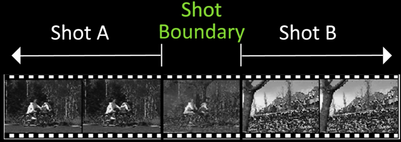
Shot boundary detection
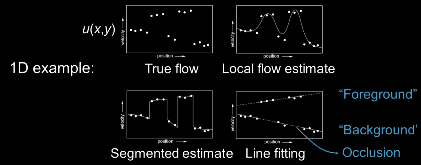
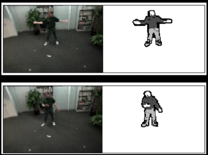
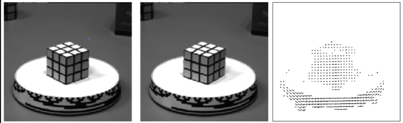
Motion segmentation
- Segment the video into multiple coherently moving objects

Motion and perceptual organization
Gestalt psychology (Wertheimer, 1880-1943)
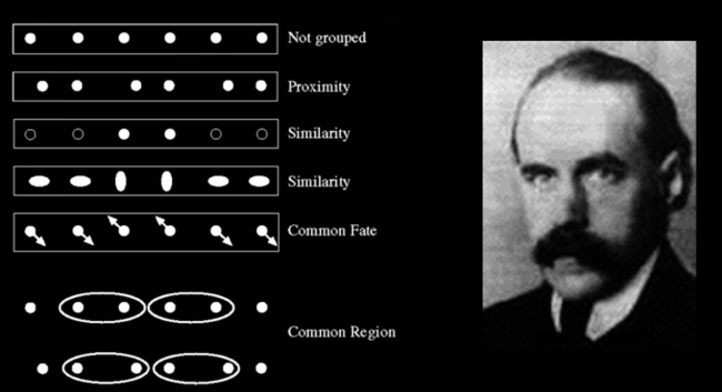
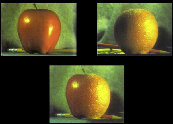
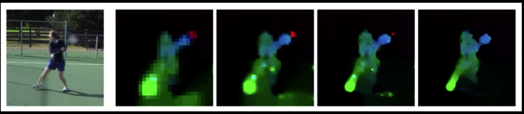
Fig.3(a) Sometimes, motion is the only cue
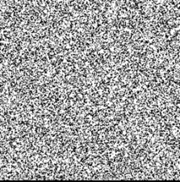
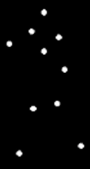
Impverished Motion
- Even "impoverished" motion data can evoke a strong percept


Motion Estimation Techniques
Featured-based methods
- Extract visual features (corners, textured areas) and track them over multiple frames
- Sparse motion fields, but more robust tracking
- Suitable when image motion is large (10s of pixels)
Direct, dense methods
- Directly recover image motion at each pixel from spatio-temporal image brightness variations
- Dense motion fields, but sensitive to appearance variations
- Suitable for video and whn image motion is small
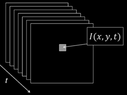
Problem Definition: Optical Flow
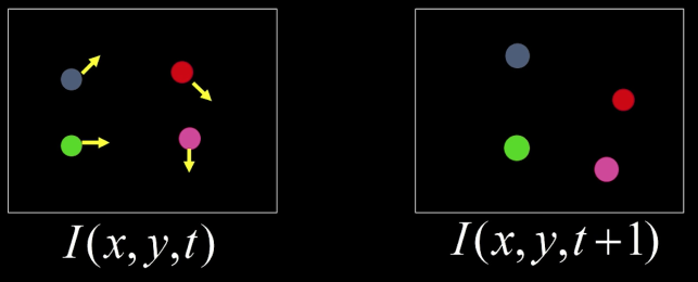
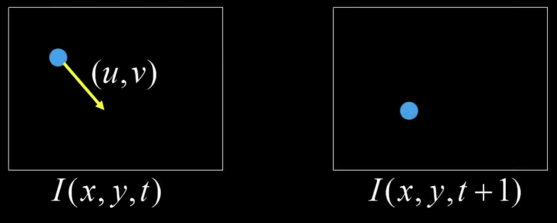
How to estimate pixel motion from image $\color{blue}{I(x,y,t)}$ to $\color{blue}{I(x,y,t+1)}$?
-> Solve pixel correspondence problem
- Given a pixel in $\color{blue}{I(x,y,t)}$, look for nearby pixels of the same color in $\color{blue}{I(x,y,t+1)}$
This is the optic flow problem
- Color constancy: a point in $\color{blue}{I(x,y,t)}$ looks the same in $\color{blue}{I(x',t',t+1)}$
- For grayscale images, this is the brightness constancy
- Small motion: points do not move very far
Optical flow constraints (grayscale images)
1) Brightness constancy constraint (equation) $$\color{blue}{I(x,y,t) = I(x+u,y+v,t+1)}$$ $$\color{blue}{0 = I(x+u,y+v,t+1)-I(x,y,t)}$$
2) Small motion: (u and v are less than 1 pixel, or smooth)
Taylor series expansion of $I$:
$$\color{blue}{I(x+u,y+v) = I(x,y) + \frac{\partial I}{\partial x}u + \frac{\partial I}{\partial y}v + [higher\, order\, terms]}$$ $$\color{blue}{I(x+u,y+v) \approx I(x,y) + \frac{\partial I}{\partial x}u + \frac{\partial I}{\partial y}v}$$
Combining these two equations:
$$\color{blue}{0 = I(x+u,y+v,t+1)-I(x,y,t)}$$ $$\color{blue}{0 \approx I(x,y,t+1)-I_xu + I_yv - I(x,y,t)}$$
$\color{blue}{I_x}$: = $\color{blue}{\frac{\partial I}{\partial x}}$ for $\color{blue}{t}$ or $\color{blue}{t+1}$
$$\color{blue}{0 \approx [I(x,y,t+1)- I(x,y,t)]+I_xu + I_yv }$$ $$\color{blue}{0 \approx I_t+I_xu + I_yv }$$
$$\color{blue}{I_t + \nabla I \cdot <u,v>}$$ $$\color{blue}{\implies 0 \approx I_t + \nabla I \cdot <u,v>}$$ In the limit as $\color{blue}{u}$ and $\color{blue}{v}$ approaches zero, this becomes exact: $$\color{blue}{0 = I_t + \nabla I \cdot <u,v>}$$
Brightness constancy constraint equation
$$\color{blue}{I_xu + I_yv + I_t = 0}$$
Gradient Component of Flow
Q: How many unknowns and equations per pixel?
2 unknown(u,v) but 1 equaton
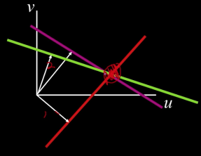
Intuitively, what does this constraint mean?
- The component of the flow in the gradient direction is determined
- The component of the flow parallel to an edge is unknown

Aperture problem

Gradient component of flow
Some falks say: "This explains the Barber Pole illusion"
http://www.sandlotscience.com/Ambiguous/Barberpole_Illusion.htm
http://www.liv.ac.uk/~marcob/Trieste/barberpole.html
Additinal Flow Constraints Quize
What additional constraints you can use:
- Nearby pixels move together
- Motion must be consistent over the entire image
- Only consider distinct regions
Smooth Optical Flow (Horn and Schunck - long ago)
- Formulate Error in Optical Flow Constraint:
$$\color{blue}{e_c = \int \int_{image} (I_xu+I_yv+I_t)^2dxdy}$$
We need additional constraints (pardon the integrals)
Smoothness constraint: motion field tends to vary smoothly over the image
$$\color{blue}{e_s= \int \int_{image} (u_x^2 + u_y^2)+(v_x^2 + v_y^2)dxdy}$$
- Penalized for changes in $\color{blue}{u}$ and $\color{blue}{v}$ over the image
Given both terms, find $\color{blue}{(u,v)}$ at each image point that minimizes:
$$\color{blue}{e=e_s+\lambda e_c}$$
$\color{blue}{\lambda}$: weighting factor
I kind of looked like Megan as I was typing the notes for this lesson (recording with no interest and no idea whatsoever of what Aaron is talking about). Let's hope the king charges me back with stormlight power and excitement as Barcelona faces Madrid in the copa del rey tomorrow
Solving the Aperture Problem
Basic idea: Impose local constraints to get more equations for a pixel:
- E.g. assume that the flow field is smooth locally
One method: pretend the pixel's neighbors have the same $\color{blue}{(u,v)}$
- If we use a 5X5 window, that gives us 25 equations per pixel!
$$\color{blue}{0 = I_t(p_i)+\nabla I(p_i)\cdot[u\,v]}$$
$$\color{blue}{A_{25\times2} \times d_{2\times1} = b_{25\times1}}$$
$$\color{blue}{\begin{bmatrix}I_x(p_1) & I_y(p_1)\\I_x(p_2) & I_y(p_2)\\.&.\\.&.\\.&.\\I_x(p_25) & I_y(p_25)\end{bmatrix}\begin{bmatrix}u\\v\end{bmatrix} = - \begin{bmatrix}I_t(p_1)\\I_t(p_2)\\.\\.\\.\\I_t(p_25)\end{bmatrix}}$$
Lukas-Kanade flow
Problem: We have more equations than unknowns
$\color{blue}{(d = [u\, v])}$
Solution: Least squares problem
The summations are over all pixels in the $K \times K$ window
$$\color{blue}{A_{25\times2} \times d_{2\times1} = b_{25\times1} \rightarrow minimize ||Ad -b||^2}$$
$$\color{blue}{(A^TA)_{2\times2} d_{2\times1} = A^Tb_{2\times1}}$$
$$\color{blue}{\begin{bmatrix}\sum I_xI_x&\sum I_xI_y\\\sum I_xI_y&\sum I_yI_y\end{bmatrix}\begin{bmatrix}u\\v\end{bmatrix} = - \begin{bmatrix}\sum I_xI_t \\ \sum I_yI_t\end{bmatrix}}$$
Aperture Problem and Normal Flow

The gradient constraints
$$\color{blue}{I_xu + I_yv + I_t = 0}$$ $$\color{blue}{\nabla I \cdot \vec{U} + I_t = 0}$$
Combining Local Constraints
$$\nabla I^1 \cdot U = -I_t^1$$ $$\nabla I^2 \cdot U = -I_t^2$$ $$\nabla I^3 \cdot U = -I_t^3$$
When is This Solvable?
$$\color{blue}{\begin{bmatrix}\sum I_xI_x&\sum I_xI_y\\\sum I_xI_y&\sum I_yI_y\end{bmatrix}\begin{bmatrix}u\\v\end{bmatrix} = - \begin{bmatrix}\sum I_xI_t \\ \sum I_yI_t\end{bmatrix}}$$
- $\color{blue}{A^TA}$ should be invertible
- => So $\color{blue}{A^TA}$ should be well-conditioned $\color{blue}{-\frac{\lambda_1}{\lambda_2}}$ should not be too large ($\color{blue}{\lambda_1 }$= larger eigenvalue)
Eigenvectors of $A^TA$
$$\color{blue}{A^TA = \begin{bmatrix}\sum I_xI_x&\sum I_xI_y\\\sum I_xI_y&\sum I_yI_y\end{bmatrix} = \sum \begin{bmatrix}I_x\\I_y\end{bmatrix} \begin{bmatrix}I_x&I_y\end{bmatrix} = \sum \nabla I(\nabla I)^T}$$
- Also $\color{blue}{A^TA}$ should be solvable when there is no aperture problem
- Does this remind you of something???
- Recall the Harris corner detector:
- $\color{blue}{M = A^TA}$ is the second moment matrix
- The eigenvectors and eigenvalues of M relate to edge direction and magnitued
- Recall the Harris corner detector:
- Does this remind you of something???
import numpy as np
import cv2
from matplotlib import pyplot as plt
import PIL
from io import BytesIO
from IPython.display import clear_output, Image as NoteImage, display
def imshow(im,fmt='jpeg'):
    #a = np.uint8(np.clip(im, 0, 255))
    f = BytesIO()
    PIL.Image.fromarray(im).save(f, fmt)
    display(NoteImage(data=f.getvalue()))
def imread(filename):
    img = cv2.imread(filename)
    img = cv2.cvtColor(img, cv2.COLOR_BGR2RGB)
    return img
def red(im):
    return im[:,:,0]
def green(im):
    return im[:,:,1]
def blue(im):
    return im[:,:,2]
def gray(im):
    return cv2.cvtColor(im.copy(), cv2.COLOR_BGR2GRAY)
def square(img,center,size,color=(0,255,0)):
    y,x = center
    leftUpCorner = (x-size,y-size)
    rightDownCorner = (x+size,y+size)
    cv2.rectangle(img,leftUpCorner,rightDownCorner,color,3)
def normalize_img(s):
    start = 0
    end = 255
    width = end - start
    res = (s - s.min())/(s.max() - s.min()) * width + start
    return res.astype(np.uint8)
def line(img,x):
    cv2.line(img,(0,x),(img.shape[1],x),(255,0,0),3)
def mse(imageA, imageB):
        # the 'Mean Squared Error' between the two images is the
        # sum of the squared difference between the two images;
        # NOTE: the two images must have the same dimension
        err = np.sum((imageA.astype("float") - imageB.astype("float")) ** 2)
        err /= float(imageA.shape[0] * imageA.shape[1])
        # return the MSE, the lower the error, the more "similar"
        # the two images are
        return err
def random_color():
    color = list(np.random.choice(range(256), size=3))
    return (int(color[0]),int(color[1]),int(color[2]))
## from https://sandipanweb.wordpress.com/2018/02/25/implementing-lucas-kanade-optical-flow-algorithm-in-python/
import numpy as np
from scipy import signal
def optical_flow(I1g, I2g, window_size, tau=1e-2):

    kernel_x = np.array([[-1., 1.], [-1., 1.]])
    kernel_y = np.array([[-1., -1.], [1., 1.]])
    kernel_t = np.array([[1., 1.], [1., 1.]])#*.25
    w = window_size//2 # window_size is odd, all the pixels with offset in between [-w, w] are inside the window
    I1g = I1g / 255. # normalize pixels
    I2g = I2g / 255. # normalize pixels
    # Implement Lucas Kanade
    # for each point, calculate I_x, I_y, I_t
    mode = 'same'
    fx = signal.convolve2d(I1g, kernel_x, boundary='symm', mode=mode)
    fy = signal.convolve2d(I1g, kernel_y, boundary='symm', mode=mode)
    ft = signal.convolve2d(I2g, kernel_t, boundary='symm', mode=mode) + signal.convolve2d(I1g, -kernel_t, boundary='symm', mode=mode)
    u = np.zeros(I1g.shape)
    v = np.zeros(I1g.shape)
    # within window window_size * window_size
    for i in range(w, I1g.shape[0]-w):
        for j in range(w, I1g.shape[1]-w):
            Ix = fx[i-w:i+w+1, j-w:j+w+1].flatten()
            Iy = fy[i-w:i+w+1, j-w:j+w+1].flatten()
            It = ft[i-w:i+w+1, j-w:j+w+1].flatten()

            b = np.reshape(It, (It.shape[0],1)) # get b here
            A = np.vstack((Ix, Iy)).T # get A here

            if np.min(abs(np.linalg.eigvals(np.matmul(A.T, A)))) >= tau:
                nu = np.matmul(np.linalg.pinv(A), b) # get velocity here
                u[i,j]=nu[0]
                v[i,j]=nu[1]
    return (u,v)
from PIL import Image
import imageio
def decode_gif_file(fname):
    imgs = []
    gif = imageio.mimread(fname)
    nums = len(gif)
    print("Total {} frames in the gif!".format(nums))
    # convert form RGB to BGR
    if len(gif[0].shape)>2:
        imgs = [cv2.cvtColor(img, cv2.COLOR_BGR2RGB) for img in gif]
    else:
        imgs = [im for im in gif]
    return imgs
def get_uvs(imgs,window=15):
    uvs = []
    for i in range(len(gimgs)-1):
        u,v = optical_flow(imgs[i],imgs[i+1],15)
        #u,v = np.rot90(u),np.rot90(v)
        uvs.append((u,v))
    return uvs
def draw_moving_field(uvs,imgs,selected):
    for r,im in enumerate(imgs[:-2]):
        u,v = uvs[r][0],uvs[r][1]
        for i,j in selected:
            pt = np.array([i,j])
            uv = np.array([u[i,j],v[i,j]])*4
            pt2 = ((pt + uv)).astype(np.int)
            cv2.arrowedLine(imgs[r], tuple(pt), tuple(pt2), (255,0,0), 1)
f1,t1,s1 = 0,260,10
f2,t2,s2 = 0,240,10
selected = [(i,50) for i in range(f1,t1,s1)]
for j in range(f2,t2,s2):
    selected += [(i,j) for i in range(f1,t1,s1)]

imgs = decode_gif_file("imgs/rubic.gif")
uvs_rubic = get_uvs(imgs)
## For some reason this must be flipped and rotated to work
uvs_rubic = [(np.fliplr(np.rot90(u,3)),np.fliplr(np.rot90(v,3))) for u,v in uvs_rubic]
cimgs = [cv2.cvtColor(im, cv2.COLOR_GRAY2RGB) for im in imgs]
draw_moving_field(uvs_rubic,cimgs,selected)
imageio.mimsave('imgs/rubic_rd.gif', cimgs,fps=1)
f1,t1,s1 = 0,200,8
f2,t2,s2 = 0,200,8
selected = [(i,50) for i in range(f1,t1,s1)]
for j in range(f2,t2,s2):
    selected += [(i,j) for i in range(f1,t1,s1)]

imgs = decode_gif_file("imgs/sphere.gif")
gimgs = [gray(im) for im in imgs]
uvs_sphere = get_uvs(gimgs)
## For some reason this must be flipped and rotated to work
uvs_sphere = [(np.fliplr(np.rot90(u,3)),np.fliplr(np.rot90(v,3))) for u,v in uvs_sphere]
draw_moving_field(uvs_sphere,imgs,selected)
imageio.mimsave('imgs/sphere_rd.gif', imgs,fps=1)
Quiz
When does the optical flow equation become solvable?
- $\lambda_1 \& \lambda_2$ are small
- $\lambda_1 >> \lambda_2$
- $\lambda_1 << \lambda_2$
- $\lambda_1$~$\lambda_2$ both fairly large
RGB Version
- One method: pretend the pixel's neighbors have the same $(u,v)$
$$\color{blue}{0 = I_t(p_i)[0,1,2]+\nabla I(p_i)[0,1,2]\cdot[u\,v]}$$
$$\color{blue}{A_{75\times2} \times d_{2\times1} = b_{75\times1}}$$
$$\color{blue}{\begin{bmatrix}I_x(p_1)[0] & I_y(p_1)[0]\\I_x(p_1)[1] & I_y(p_1)[1]\\I_x(p_1)[2] & I_y(p_1)[2]\\.&.\\.&.\\.&.\\I_x(p_25)[0] & I_y(p_25)[0]\\I_x(p_25)[0] & I_y(p_25)[0]\\I_x(p_25)[1] & I_y(p_25)[2]\end{bmatrix}\begin{bmatrix}u\\v\end{bmatrix} = - \begin{bmatrix}I_t(p_1)[0]\\I_t(p_1)[1]\\I_t(p_1)[2]\\.\\.\\.\\I_t(p_25)[0]\\I_t(p_25)[1]\\I_t(p_25)[2]\end{bmatrix}}$$
Note that **RGB** alone at a pixel is not enough to disambiguate because R,G & B are correlated. Just provides better gradient
Errors in Lucas Kanade
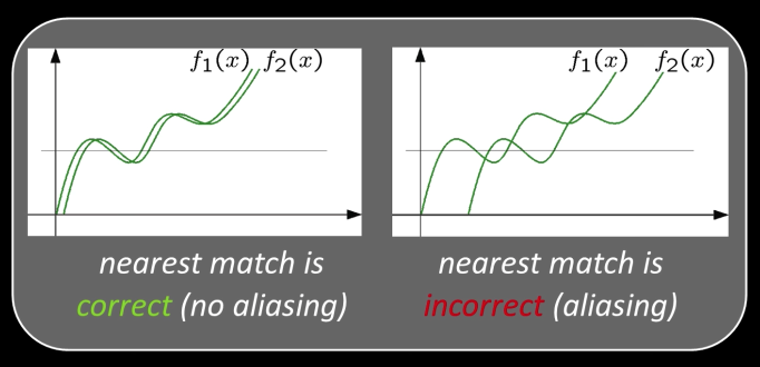
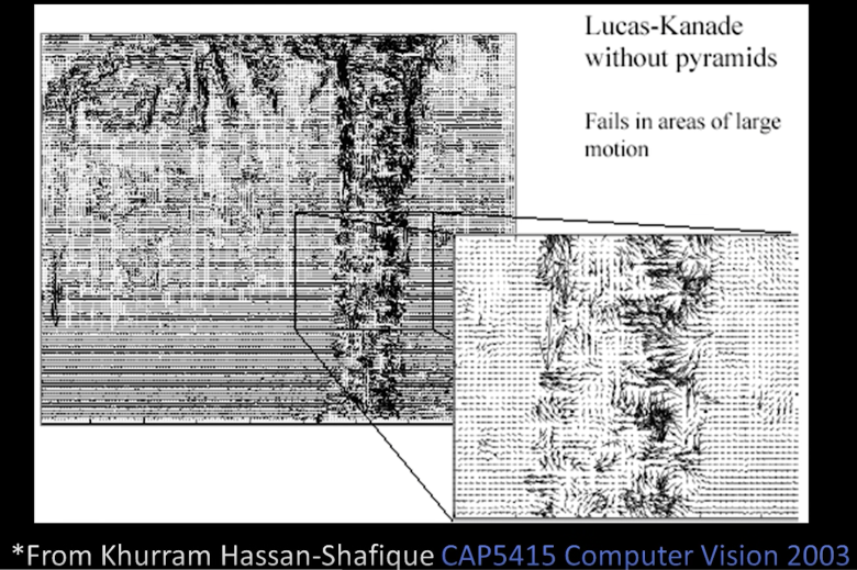
- The motion is large (larger than a pixel)- Taylor doesn't hold
- Not-linear: Iterative refinment
- Local minima: corse-to-fine estimation
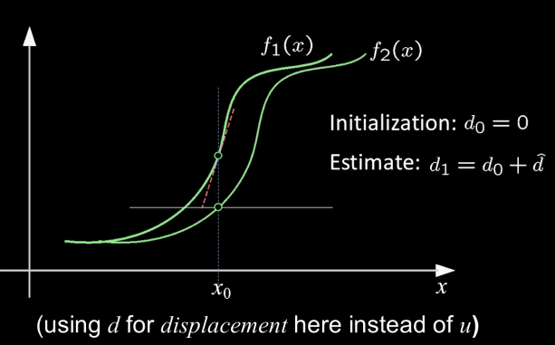
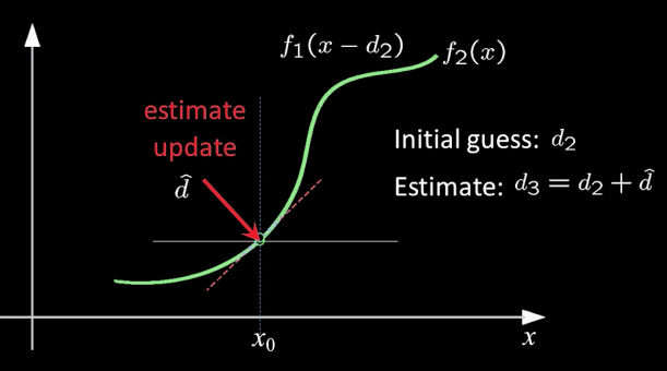
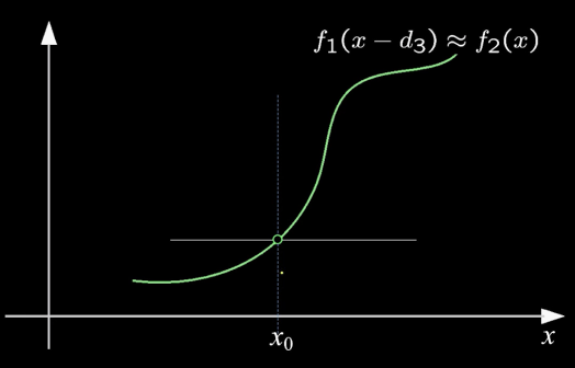
Not tangent: Iterative Refinement
Iterative Lukas-Kanade Algorithm
- Estimate velocity at each pixel by solving Lucas-Kanade equations
- Warp $I_t$ towards $I_{t+1}$ using the estimated flow field
- Use image warping techniques
- Repeat until convergence
Optical Flow: Iterative Estimation

Implementation Issues
- Warping is not easy (ensure that errors in warping are smaller than the estimate refinement)- but it is in Matlab
- Often useful to low-pass filter the images before motion estimation (for better derivative estimation, and linear approximations to image intensity)
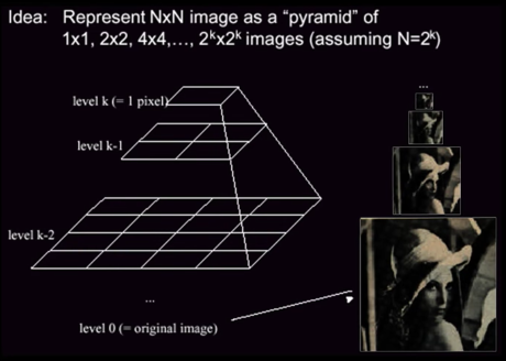
Reduce the Resolution
Is the below motion is small enough to run Lucas-Kanade?!
- Propably not much larger than one pixel. An entire tree is covered
- How might we solve this problem?
## From L2
def resize(image,size):
    return cv2.resize(image, size)
img = imread("imgs/L634.png")
imshow(resize(img[::2,::2],(img.shape[1],img.shape[0])))
imshow(resize(img[::4,::4],(img.shape[1],img.shape[0])))
imshow(resize(img[::8,::8],(img.shape[1],img.shape[0])))


Filter and then subsampling
from skimage.filters import gaussian as gaussian_filter
imshow(img)
gimg = img.copy()
for i in range(3):
    gimg = normalize_img(gaussian_filter(gimg, sigma=2,multichannel=True)).astype(np.uint8)
    gimg = gimg[::2,::2]
    imshow(resize(gimg,(img.shape[1],img.shape[0])))


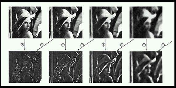


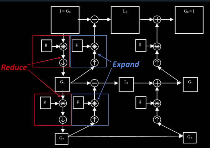
Reduce and Expand


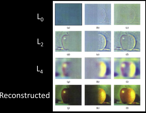
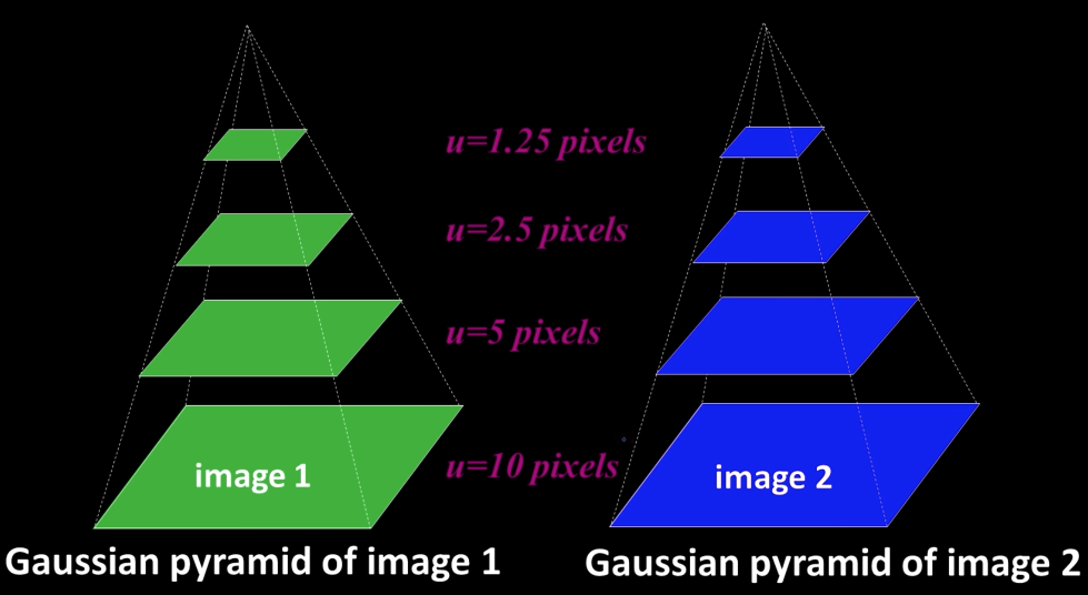
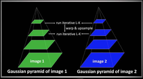
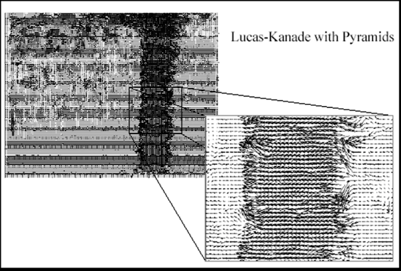
Hierarchical LK

Hierarchical LK
- Compute Iterative LK at level K
- Initialize $\color{blue}{u_{K+1}, v_{K+1} = 0}$ at size of level $\color{blue}{K+1}$
For each level $\color{blue}{i}$ from $\color{blue}{K}$ to 0
- Upsample (EXPAND) $\color{blue}{u_{i+1},v_{i+1}}$ to create $\color{blue}{u_i^p,v_i^p}$ flow fields of now twice resolution as level $\color{blue}{i+1}$
- Multiply $\color{blue}{u_i^p,v_i^p}$ by 2 to get predicted flow
- Warp level $\color{blue}{i}$ Gaussian version of $\color{blue}{I_2}$ according to predicted flow to create $\color{blue}{I'_2}$
Apply LK between $\color{blue}{I_2'}$ and level $\color{blue}{i}$ Gaussian version of $I_1$ to get $\color{blue}{u_i^\delta, v_i^\delta}$ (the correction in flow)
Add corrections to obtain the flow $\color{blue}{u_i,v_i}$ at $\color{blue}{i^{th}}$ level, i.e.,$$\color{blue}{u_i = u_i^p + u_i^\delta}$$ $$\color{blue}{v_i = v_i^p + v_i^\delta}$$
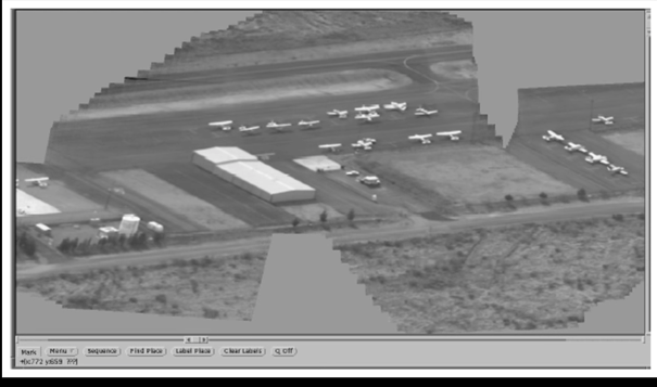
Optical Flow Results
Sparse LK
- The Lucas-Kanade algorithm described gives a dense field, $(u,v)$ everywhere
- But we said that we only want to solve LK where the eigenvalues are well behaved
- "Sparse LK" is basically just that: hierarchical applied to good feature locations
- OpenCV LK used to be dense - then became sparse
Start with Something Similar to Lucas Kanade
- gradient constancy
- energy minimization with smoothing term
- region matching
- keypoint matching (long-range)
# """
# Run the following code in the terminal so you can exit gracefully.
# Source: https://pysource.com/2018/05/14/optical-flow-with-lucas-kanade-method-opencv-3-4-with-python-3-tutorial-31/

# The tutorial shows how to use Lucas-Kanade method implemeted on opencv to follow the movement of a pencil head.
# """

# import cv2
# import numpy as np

# cap = cv2.VideoCapture(0)

# # Create old frame
# _, frame = cap.read()
# old_gray = cv2.cvtColor(frame, cv2.COLOR_BGR2GRAY)

# # Lucas kanade params
# lk_params = dict(winSize = (15, 15),
#                  maxLevel = 4,
#                  criteria = (cv2.TERM_CRITERIA_EPS | cv2.TERM_CRITERIA_COUNT, 10, 0.03))

# # Mouse function
# def select_point(event, x, y, flags, params):
#     global point, point_selected, old_points
#     if event == cv2.EVENT_LBUTTONDOWN:
#         point = (x, y)
#         point_selected = True
#         old_points = np.array([[x, y]], dtype=np.float32)

# cv2.namedWindow("Frame")
# cv2.setMouseCallback("Frame", select_point)

# point_selected = False
# point = ()
# old_points = np.array([[]])
# while True:
#     _, frame = cap.read()
#     gray_frame = cv2.cvtColor(frame, cv2.COLOR_BGR2GRAY)

#     if point_selected is True:
#         cv2.circle(frame, point, 5, (0, 0, 255), 2)

#         new_points, status, error = cv2.calcOpticalFlowPyrLK(old_gray, gray_frame, old_points, None, **lk_params)
#         old_gray = gray_frame.copy()
#         old_points = new_points

#         x, y = new_points.ravel()
#         cv2.circle(frame, (x, y), 5, (0, 255, 0), -1)


#     cv2.imshow("Frame", frame)

#     key = cv2.waitKey(1)
#     if key == 27:
#         break

# cap.release()
# cv2.destroyAllWindows()
🐐 Charming...Thank you Lucas and Kanade. I am flying to Lyon to watch the GOAT. Hope to see him at his best 🐐
import numpy as np

messi = imread('imgs/messi.jpg')
graymessi = gray(messi)
rows,cols = graymessi.shape

M = np.float32([[1,0,100],[0,1,50]])
dst = cv2.warpAffine(graymessi,M,(cols,rows))
imshow(graymessi)
imshow(dst)


M = cv2.getRotationMatrix2D((cols/2,rows/2),45,1)
dst = cv2.warpAffine(graymessi,M,(cols,rows))
imshow(dst)

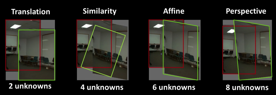
pts1 = np.float32([[50,50],[200,50],[50,200]])
pts2 = np.float32([[10,100],[200,50],[100,250]])
M = cv2.getAffineTransform(pts1,pts2)
dst = cv2.warpAffine(graymessi,M,(cols,rows))
imshow(dst)

# the points are not meant for messi image, check the one in the link
# https://docs.opencv.org/3.0-beta/doc/py_tutorials/py_imgproc/py_geometric_transformations/py_geometric_transformations.html
pts1 = np.float32([[56,65],[368,52],[28,387],[389,390]])
pts2 = np.float32([[0,0],[300,0],[0,300],[300,300]])
M = cv2.getPerspectiveTransform(pts1,pts2)
dst = cv2.warpPerspective(graymessi,M,(cols,rows))
imshow(dst)


Full motion model
From physics or elsewhere:
$$\color{blue}{V = \Omega \times R = T}$$ $$\color{blue}{\begin{bmatrix}V_X\\V_Y\\V_Z\end{bmatrix}= \begin{bmatrix}0&-\omega_Z&\omega_Y\\\omega_Z&0&-\omega_X\\-\omega_Y&\omega_X&0\end{bmatrix} \begin{bmatrix}X\\Y\\Z\end{bmatrix} + \begin{bmatrix}V_{T_X}\\V_{T_Y}\\V_{T_Z}\end{bmatrix}}$$
$\color{blue}{\begin{bmatrix}V_X\\V_Y\\V_Z\end{bmatrix}}$ velocity vector
$\color{blue}{\begin{bmatrix}V_{T_X}\\V_{T_Y}\\V_{T_Z}\end{bmatrix}}$ Translational Component of Velocity
$\color{blue}{\begin{bmatrix}\omega_X\\\omega_Y\\\omega_Z\end{bmatrix}}$ Angular Velocity
General Motion
$$\color{blue}{x = f \frac{X}{Z}}$$ $$\color{blue}{y = f \frac{Y}{Z}}$$
$$\color{blue}{u = v_x = f\frac{ZV_X-XV_Z}{Z^2} = f\frac{V_X}{Z}-\left(f\frac{X}{Z}\right)\frac{V_Z}{Z}= f\frac{V_X}{Z}-x\frac{V_Z}{Z}}$$
$$\color{blue}{v = v_y = f\frac{ZV_Y-YV_Z}{Z^2} = f\frac{V_Y}{Z}-\left(f\frac{Y}{Z}\right)\frac{V_Z}{Z}= f\frac{V_Y}{Z}-y\frac{V_Z}{Z}}$$
$$\color{blue}{\begin{bmatrix}u(x,y)\\v(x,y)\end{bmatrix} = \frac{1}{Z(x,y)} A(x,y)T + B(x,y)\Omega}$$
Where $T$ is the translation vector, $\Omega$ is rotation
$$\color{blue}{A(x,y) = \begin{bmatrix}-f&0&x\\0&-f&y\end{bmatrix}}$$
$$\color{blue}{B(x,y) = \begin{bmatrix}\frac{xy}{f}&\frac{-(f+x^2)}{f} & y\\\frac{f+y^2}{f}&\frac{-(xy)}{f} & -x\end{bmatrix}}$$
Why the Z(x,y) is only in the translation component?
because it only matters when the image plane is moving. When the image plane is rotating the depth doesn't matter.
Motion of a Plane
If a plane and perspective
$$\color{blue}{aX + bY + cZ + d = 0}$$
$$\color{blue}{u(x,y) = a_1 + a_2x + a_3y + a_7x^2 + a_8xy}$$ $$\color{blue}{v(x,y) = a_4 + a_5x + a_6y + a_7xy + a_8y^2}$$
If a plane and orthographic...
$$\color{blue}{u(x,y) = a_1 + a_2x + a_3y }$$
$$\color{blue}{v(x,y) = a_4 + a_5x + a_6y }$$
Affine Motion

$$\color{blue}{u(x,y) = a_1 + a_2x + a_3y }$$ $$\color{blue}{v(x,y) = a_4 + a_5x + a_6y }$$
Substituting into the brightness constancy equation:
$$\color{blue}{I_x\cdot u + I_y\cdot v + I_t \approx 0}$$
$$\color{blue}{I_x(a_1+a_2x+a_3y) + I_y(a_4+a_5x+a_6y) + I_t \approx 0}$$
- Each pixel provides 1 linear constraint in 6 unknowns
- Least squares minimization:
$$\color{blue}{Err(\vec{a}) = \sum[I_x(a_1+a_2x+a_3y) + I_y(a_4+a_5x+a_6y) + I_t]^2}$$
Can sum gradients over window or entire image: $$\color{blue}{Err(\vec{a}) = \sum[I_x(a_1+a_2x+a_3y) + I_y(a_4+a_5x+a_6y) + I_t]^2}$$
Minimize squared error (robustly)
$$\color{blue}{\begin{bmatrix} I_x&I_xX_1&I_xy_1&I_y&I_yx_1&I_yy_1\\ I_x&I_xX_2&I_xy_2&I_y&I_yx_2&I_yy_2\\ .\\ .\\ .\\ I_x&I_xX_n&I_xy_n&I_y&I_yx_n&I_yy_n\\ \end{bmatrix} \cdot \begin{bmatrix}a_1\\a_2\\a_3\\a_4\\a_5\\a_6\end{bmatrix} = - \begin{bmatrix}I_t^1\\I_t^1\\.\\.\\.\\I_t^n\end{bmatrix} }$$
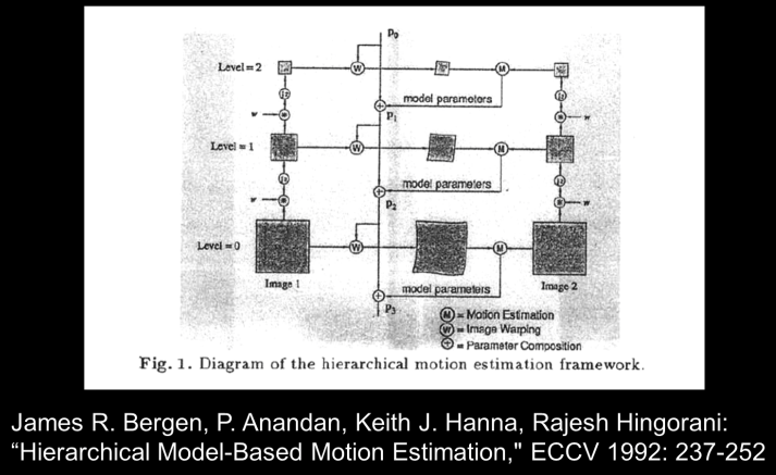
Hierarchical model-based flow
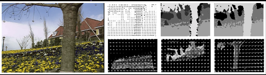
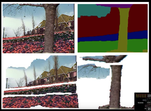
Layered Motion
Basic idea: break image sequence into "layers" each of which has a coherent motion
What are layers?
Each layer is defined by an alpha mask and an affine motion model

Equation of a plane (parameters $a_1,a_2,a_3$ can be found by least squares)