=====================================

5A - L1 Photometry

=====================================

Photometry

Measuring light

Fig.1 (a): The lighting hit the scene and get reflected to the camera according the physical models and the processed image in the camera get stored in the computer

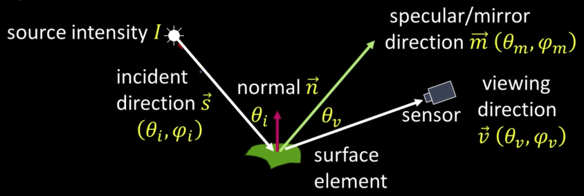
Lights, surface, and shadows

Fig.1 (b): The surface on the road is clearly a shadow and not a texture. But it might have been painted and your brain was tricked

Reflections

Fig.1 (c): The image on the right looks like a reflection. The image on the left is also look like a reflection but a little bit distorted because of the glass

Refraction

Fig.1 (d): Refraction is mostly seen in water or deformed glass. The image on the right has both reflection and refraction

Interreflection

Fig.1 (e): As light bounces around, objects get reflected in-between surfaces

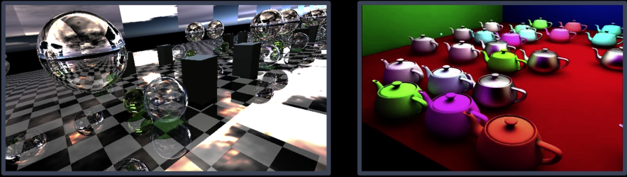
Scattering

Fig.1 (f): the impact of moisture or any other factor on the image that enter the eye or the camera

Surface Appearance

Fig.2

• Image intensity = $f$(normal, surface reflectance, illumination)
• Surface reflection depends on both the viewing and illumination direction

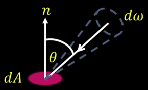
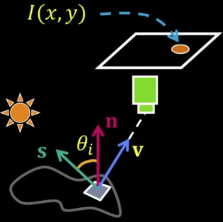
Radiometry Radiance

Radiance(L): Energy carried by a ray
- Power per unit area perpendicular to direction of travel, per unit solid angle
- Units: Watts per square meter per steradian ($Wm^{-2}sr^{-1}$)

Fig.3 (a)

Radiometry Irradiance

Irradiance(E): Energy arriving at a surface
- Incident power in a given direction, per unit area
- Units: $Wm^{-2}$

Fig.3(b)

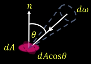
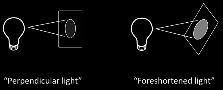
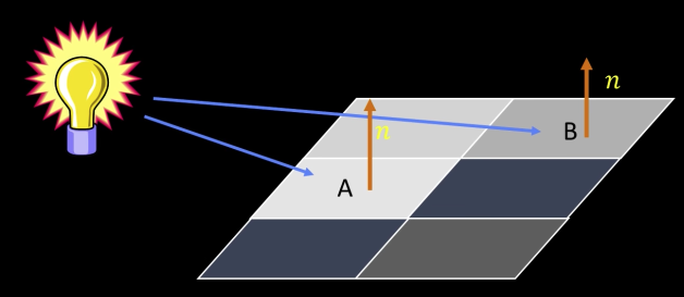
Foreshortening: A simple observation

Fig.3(c) if the card was perpendicular (left), a certain amout of light will fall on it. If it was telted (right), than that amount will get spread over larger area, and thus we get less light per unit area from that light source

For a surface receiving radiance $L(\theta, \varphi)$coming in from $d\omega$ the corresponding irradiance is

$$E(\theta,\varphi) = L(\theta,\varphi)cos(\theta) d\omega$$

BRDF: Bidirectional Reflectance Distribution Function

Fig.4

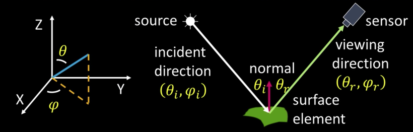
Irradiance: Light per unit area incident on a surface

Radiance: Light from the surface reflected in a given direction, within a given solid angle

$E^{surface}(\theta_i,\varphi_i)$ : Irradiance at surface from direction $(\theta_i,\varphi_i)$

$L^{surface}(\theta_i,\varphi_i)$ : Rradiance from surface in direction $(\theta_r,\varphi_r)$

BRDF: $f(\theta_i,\varphi_i;\theta_r,\varphi_r) = \frac{L^{surface}(\theta_i,\varphi_i)}{E^{surface}(\theta_i,\varphi_i)}$

Important properties of BRDFs

• Helmholts Reciprocity:

$f(\theta_i,\varphi_i;\theta_r,\varphi_r) = f(\theta_r,\varphi_r;\theta_i,\varphi_i)$

• Rotational Symmetry (Isotropy):

$f(\theta_i,\varphi_i;\theta_r,\varphi_r) = f(\theta_i,\theta_r;\varphi_i - \varphi_r)$

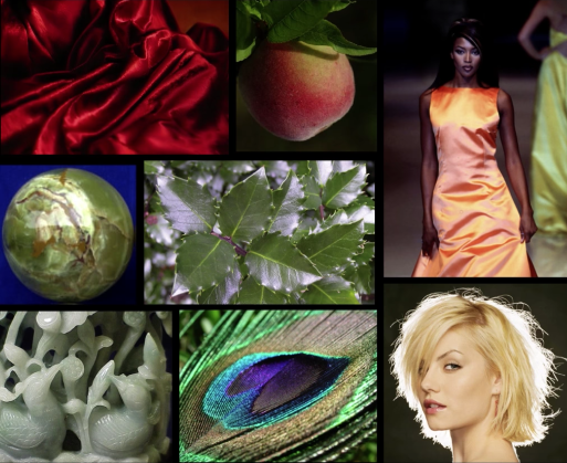
BRDF's can be incredibly complicated

Fig.5

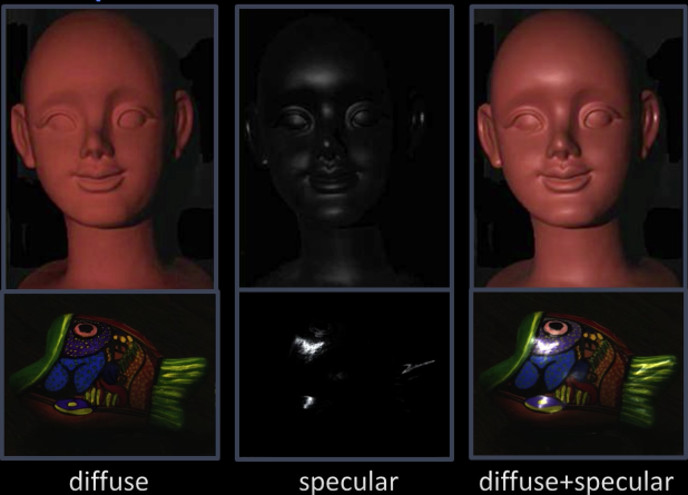
Reflection Models

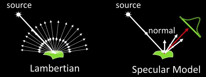
**Body (diffuse) Reflection:** - Diffuce Reflection - Matte Appearance - Non-Homogeneous medium - Clay, paper, etc.

Fig.5(b) Surface reflection

**Surface reflection:** - Specular Reflection - Glossy Appearance - Highlights - Dominant for Metals

Fig.5(a) Diffuse reflection

Fig.5(c) Image Intensity

Image Intensity = Body Reflection + Surface Reflection

Diffuse Reflection and Lambertian BTDF

• Only body reflection, and no specular reflection
• Lamberts law - essentially a patch looks equally bright from every direction

Fig.6 (a) The more perpendicular the light is the more light you have reflected out, but the amount of light comming out in each direction is not the same.

Fig.6 (b) The amount of area that can be seen in the surface grows by 1/cosine of the angle. So, as the angle gets closer and closer to 90 degrees, infinit amount of patch will be seen for the same pixel

Diffuse Reflection and Lamertian BRDF

Fig.7

• Surface appears equally bright from all directions! (independent of $\overrightarrow{v})$

• Lambertian BRDF is simply a constant - the albedo:

$$\color{blue}{f(\theta_i,\varphi_i;\theta_r,\varphi_r) = \rho_d}$$

• Surface Radiance:

$$\color{blue}{L = \rho_d I cos(\theta_i) = \rho_d I (\overrightarrow{n}\cdot \overrightarrow{s})}$$

Where:

$\color{blue}{I}$: source intensity

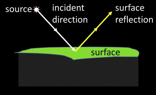
Specular Reflection and Mirror BRDF

How about a mirror?

Reflection only at mirror angle

Fig.8

• All incident light reflected in a single direction (visible when $\overrightarrow{v} = \overrightarrow{m}$)

• Mirror BRDF is simple a double-delta function:

$$\color{blue}{f(\theta_i,\varphi_i;\theta_r,\varphi_r) = \rho_s \delta(\theta_i - \theta_v)\delta(\phi_i + \pi - \phi_v)}$$

• Surface Radiance: $$\color{blue}{L = I \rho_s \delta(\theta_i - \theta_v)\delta(\varphi_i + \pi - \varphi_v)}$$

$\color{blue}{L = I \rho_s \delta(\overrightarrow{m} = \overrightarrow{v}) }$ or $\color{blue}{I \rho_s \delta(\overrightarrow{n} = \overrightarrow{h})}$
$\color{blue}{\overrightarrow{h}}$ is the "half angle"

Specular Reflection and Glossy BRDF

Fig.9(a)

$$L = I \rho_s (\overrightarrow{m}\cdot \overrightarrow{v})^k$$

Fig.9(b)

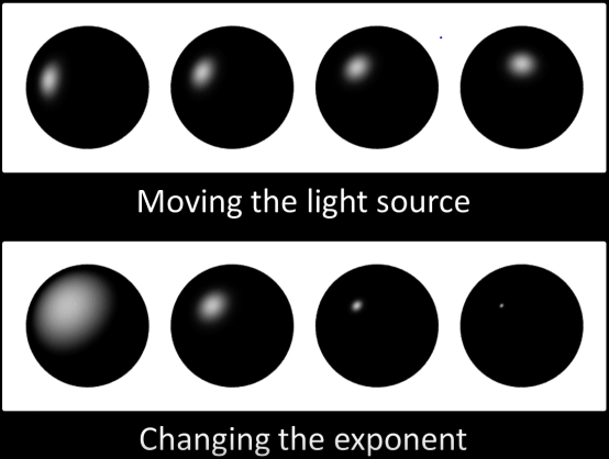
Phong Reflection Model

The BRDF of many surfaces can be approximated by:

Lambertian + Specular Model

Fig.10

import numpy as np
import cv2
from matplotlib import pyplot as plt
import PIL
from io import BytesIO
from IPython.display import clear_output, Image as NoteImage, display
def imshow(im,fmt='jpeg'):
    #a = np.uint8(np.clip(im, 0, 255))
    f = BytesIO()
    PIL.Image.fromarray(im).save(f, fmt)
    display(NoteImage(data=f.getvalue()))
def imread(filename):
    img = cv2.imread(filename)
    img = cv2.cvtColor(img, cv2.COLOR_BGR2RGB)
    return img
def red(im):
    return im[:,:,0]
def green(im):
    return im[:,:,1]
def blue(im):
    return im[:,:,2]
def gray(im):
    return cv2.cvtColor(im, cv2.COLOR_BGR2GRAY)
def square(img,center,size,color=(0,255,0)):
    y,x = center
    leftUpCorner = (x-size,y-size)
    rightDownCorner = (x+size,y+size)
    cv2.rectangle(img,leftUpCorner,rightDownCorner,color,3)
def normalize_img(s):
    start = 0
    end = 255
    width = end - start
    res = (s - s.min())/(s.max() - s.min()) * width + start
    return res.astype(np.uint8)
def line(img,x):
    cv2.line(img,(0,x),(img.shape[1],x),(255,0,0),3) 
def mse(imageA, imageB):
        # the 'Mean Squared Error' between the two images is the
        # sum of the squared difference between the two images;
        # NOTE: the two images must have the same dimension
        err = np.sum((imageA.astype("float") - imageB.astype("float")) ** 2)
        err /= float(imageA.shape[0] * imageA.shape[1])
        # return the MSE, the lower the error, the more "similar"
        # the two images are
        return err
def random_color():
    color = list(np.random.choice(range(256), size=3))
    return (int(color[0]),int(color[1]),int(color[2]))

## Code from https://gist.github.com/rossant/6046463


import numpy as np
import matplotlib.pyplot as plt
from PIL import Image

w = 400
h = 300

def normalize(x):
    x /= np.linalg.norm(x)
    return x

def intersect_plane(O, D, P, N):
    # Return the distance from O to the intersection of the ray (O, D) with the 
    # plane (P, N), or +inf if there is no intersection.
    # O and P are 3D points, D and N (normal) are normalized vectors.
    denom = np.dot(D, N)
    if np.abs(denom) < 1e-6:
        return np.inf
    d = np.dot(P - O, N) / denom
    if d < 0:
        return np.inf
    return d

def intersect_sphere(O, D, S, R):
    # Return the distance from O to the intersection of the ray (O, D) with the 
    # sphere (S, R), or +inf if there is no intersection.
    # O and S are 3D points, D (direction) is a normalized vector, R is a scalar.
    a = np.dot(D, D)
    OS = O - S
    b = 2 * np.dot(D, OS)
    c = np.dot(OS, OS) - R * R
    disc = b * b - 4 * a * c
    if disc > 0:
        distSqrt = np.sqrt(disc)
        q = (-b - distSqrt) / 2.0 if b < 0 else (-b + distSqrt) / 2.0
        t0 = q / a
        t1 = c / q
        t0, t1 = min(t0, t1), max(t0, t1)
        if t1 >= 0:
            return t1 if t0 < 0 else t0
    return np.inf

def intersect(O, D, obj):
    if obj['type'] == 'plane':
        return intersect_plane(O, D, obj['position'], obj['normal'])
    elif obj['type'] == 'sphere':
        return intersect_sphere(O, D, obj['position'], obj['radius'])

def get_normal(obj, M):
    # Find normal.
    if obj['type'] == 'sphere':
        N = normalize(M - obj['position'])
    elif obj['type'] == 'plane':
        N = obj['normal']
    return N
    
def get_color(obj, M):
    color = obj['color']
    if not hasattr(color, '__len__'):
        color = color(M)
    return color

def trace_ray(rayO, rayD):
    # Find first point of intersection with the scene.
    t = np.inf
    for i, obj in enumerate(scene):
        t_obj = intersect(rayO, rayD, obj)
        if t_obj < t:
            t, obj_idx = t_obj, i
    # Return None if the ray does not intersect any object.
    if t == np.inf:
        return
    # Find the object.
    obj = scene[obj_idx]
    # Find the point of intersection on the object.
    M = rayO + rayD * t
    # Find properties of the object.
    N = get_normal(obj, M)
    color = get_color(obj, M)
    toL = normalize(L - M)
    toO = normalize(O - M)
    # Shadow: find if the point is shadowed or not.
    l = [intersect(M + N * .0001, toL, obj_sh) 
            for k, obj_sh in enumerate(scene) if k != obj_idx]
    if l and min(l) < np.inf:
        return
    # Start computing the color.
    col_ray = ambient
    # Lambert shading (diffuse).
    col_ray += obj.get('diffuse_c', diffuse_c) * max(np.dot(N, toL), 0) * color
    # Blinn-Phong shading (specular).
    col_ray += obj.get('specular_c', specular_c) * max(np.dot(N, normalize(toL + toO)), 0) ** specular_k * color_light
    return obj, M, N, col_ray

def add_sphere(position, radius, color):
    return dict(type='sphere', position=np.array(position), 
        radius=np.array(radius), color=np.array(color), reflection=.5)
    
def add_plane(position, normal):
    return dict(type='plane', position=np.array(position), 
        normal=np.array(normal),
        color=lambda M: (color_plane0 
            if (int(M[0] * 2) % 2) == (int(M[2] * 2) % 2) else color_plane1),
        diffuse_c=.75, specular_c=.5, reflection=.25)

# List of objects.
color_plane0 = 1. * np.ones(3)
color_plane1 = 0. * np.ones(3)
scene = [add_sphere([.75, .1, 1.], .6, [0., 0., 1.]),
         add_sphere([-.75, .1, 2.25], .6, [.5, .223, .5]),
         add_sphere([-2.75, .1, 3.5], .6, [1., .572, .184]),
         add_plane([0., -.5, 0.], [0., 1., 0.]),
    ]

# Light position and color.
L = np.array([5., 5., -10.])
color_light = np.ones(3)

# Default light and material parameters.
ambient = .05
diffuse_c = 1.
specular_c = 1.
specular_k = 50

depth_max = 5  # Maximum number of light reflections.
col = np.zeros(3)  # Current color.
O = np.array([0., 0.35, -1.])  # Camera.
Q = np.array([0., 0., 0.])  # Camera pointing to.
img = np.zeros((h, w, 3))

r = float(w) / h
# Screen coordinates: x0, y0, x1, y1.
S = (-1., -1. / r + .25, 1., 1. / r + .25)

# Loop through all pixels.
for i, x in enumerate(np.linspace(S[0], S[2], w)):
    if i % 50 == 0:
        print (i / float(w) * 100, "%")
    for j, y in enumerate(np.linspace(S[1], S[3], h)):
        col[:] = 0
        Q[:2] = (x, y)
        D = normalize(Q - O)
        depth = 0
        rayO, rayD = O, D
        reflection = 1.
        # Loop through initial and secondary rays.
        while depth < depth_max:
            traced = trace_ray(rayO, rayD)
            if not traced:
                break
            obj, M, N, col_ray = traced
            # Reflection: create a new ray.
            rayO, rayD = M + N * .0001, normalize(rayD - 2 * np.dot(rayD, N) * N)
            depth += 1
            col += reflection * col_ray
            reflection *= obj.get('reflection', 1.)
        img[h - j - 1, i, :] = np.clip(col, 0, 1)

0.0 %
12.5 %
25.0 %
37.5 %
50.0 %
62.5 %
75.0 %
87.5 %

img = normalize_img(img)
imshow(img)

messi400 = imread("imgs/messi400.jpg")

messi400_s = cv2.resize(messi400, dsize=(400, 300), interpolation=cv2.INTER_CUBIC)

# from L2
def resize(image,size):
    return cv.resize(image, size) 
def multiply(image,factor):
    return np.uint8(np.clip(factor*image, 0, 255))
def blend(img1,img2,factor):
    return multiply(img1,factor)+multiply(img2,1-factor)

imshow(blend(gray(messi400_s),img[:,:,0],0.4))

👑Against Eibar on past Sunday, Lionel Messi becomes first player in any of Europe's top 5 leagues to score 400 goals.👑

=====================================

5B - L1 Lightness

=====================================

• Image intensity = $f$(normal, surface reflectance, illumination)
• Surface reflection depends on both the viewing and illumination direction
  
  

  

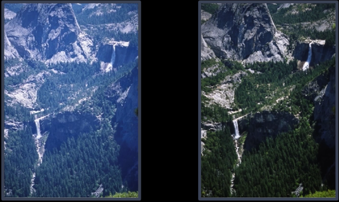
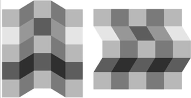
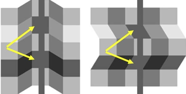
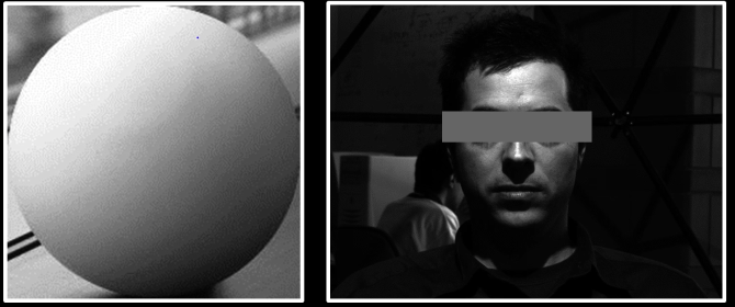
  Fig.11 What do you see??

Lightness Assumptions

Simple scene right?

Fig.12(a) You might think that square A is dark and square B is light but in fact they both have the same color

What is going on??!!

The Brain is Compensating for the "shadow"

Lightness perception is influeneced by 3D cues

Fig.12(b)

Simultaneous contrast effect

Fig.12(c)

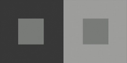
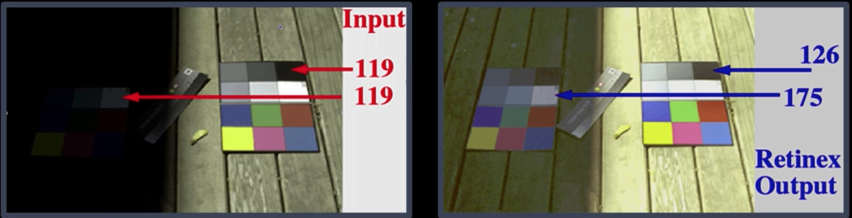
Quiz Reflectence vs Irradiance Quiz

$$\color{blue}{L(x,y) = R(x,y) * E(x,y)}$$

Where:
$\color{blue}{R(x,y)}$: surface reflectance (color, texture)
$\color{blue}{E(x,y)}$: incoming light (brintness, angle)

Which vary faster or more frequently with changes in location and which one varies slower or less frequently?

surface reflectance changes more

Ambiguity of Lighting and Reflectance

Planar, Lambertian material:

$$L = I * \rho * cos(\theta)$$

where:

$\rho$: reflectance (aka albedo)
$\theta$: angle between light and $n$
$I$: illuminance (strenght of light)

Fig.13

If we combine $\color{blue}{\theta}$ and $\color{blue}{I}$ at a point $\color{blue}{E(x,y)}$ , and have a reflectance function $\color{blue}{R(x,y)}$ then:

$$L(x,y) = R(x,y) * E(x,y)$$

The Mondrian World

Assumptions

1. Light is slowly varying
   • This is reasonable for planar world: nearby image points come from nearby scene points with same surface normal
2. Within an object reflectance is constant
3. Between objects, reflectance varies suddenly

Fig.14

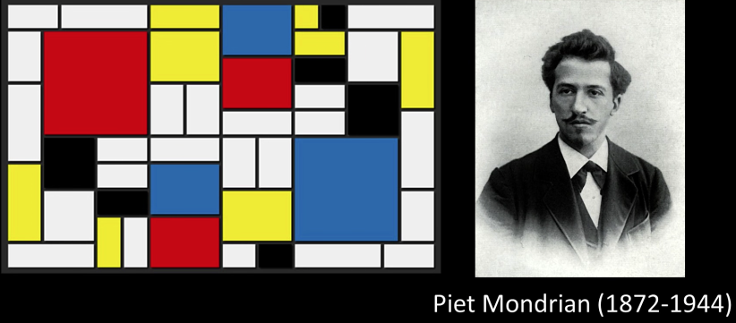
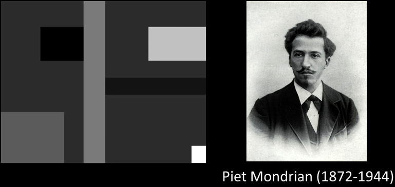
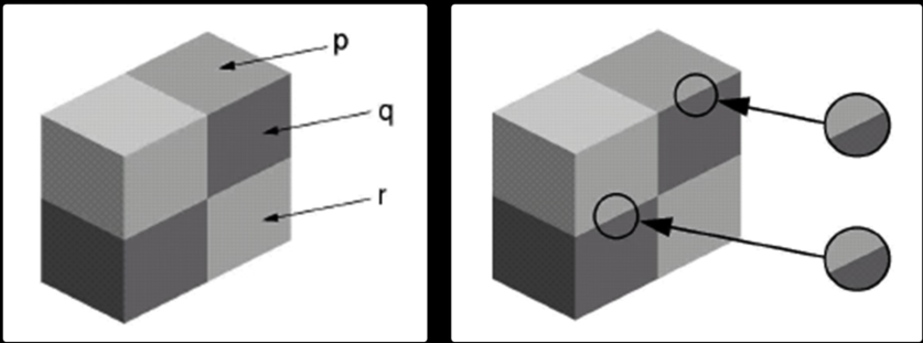
Lighning in the Mondrian World

Illumination: slowly varying

$$L(x,y) = R(x,y) * E(x,y)$$

Formally, we assume that illuminance, $\color{blue}{E}$, is low frequency

Fig.15(a) smooth illuminance

Reflectance, $\color{blue}{R}$, is constant over patches separated by edges.

Fig.15(b) sharp reflectance

Fig.15(c) Lightning

How can we recover the albedo?

We will do it in code

def display_triple(imgs,titles):
    plt.gray()
    plt.figure(figsize=(20,20))
    
    plt.subplot(131)
    ax = plt.gca()
    ax.xaxis.set_major_locator(plt.NullLocator())
    ax.yaxis.set_major_locator(plt.NullLocator())   
    plt.imshow(imgs[0])
    plt.title(titles[0], size=20)
    if len(imgs)> 1:
        plt.subplot(132)
        plt.imshow(imgs[1])
        plt.title(titles[1], size=20)
        ax = plt.gca()
        ax.xaxis.set_major_locator(plt.NullLocator())
        ax.yaxis.set_major_locator(plt.NullLocator())  
    if len(imgs)> 2:
        plt.subplot(133)
        plt.imshow(imgs[2])
        plt.title(titles[2], size=20)
        ax = plt.gca()
        ax.xaxis.set_major_locator(plt.NullLocator())
        ax.yaxis.set_major_locator(plt.NullLocator())   
    plt.show()

e = gray(imread("imgs/ch5BL1LigMonWor.png"))
r = gray(imread("imgs/ch5BL1LigMonWor2.png"))
l = blend(e,r,0.5)
display_triple([e,r,l],["Illuminance","Reflectance","Lightning"])

<Figure size 432x288 with 0 Axes>

sr = 255-r[50]
sl = 255-l[50]
se = 255-e[50]
fig,axs = plt.subplots(ncols=3)
axs[0].plot(sr)
axs[1].plot(sl)
axs[2].plot(se)

[<matplotlib.lines.Line2D at 0x1261c6198>]

Given the right chart, how to recover the left??

Retnix

Fig.16 Edwind Land

• Edwind Land (1909-1991) - inventor of Polaroid Land camera
• Early demonstrations that humans perceive different lightness (or color) for same objective brightness

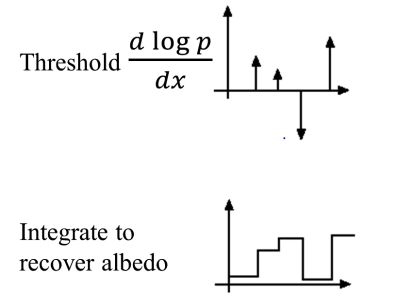
Land's Retnix Theory

• Goal: remove slow variations from the image
• Many approaches to this. One is

$$L(x,y) = R(x,y) * E(x,y)$$ $$log(L(x,y)) = log(R(x,y)) + log(E(x,y))$$

• Hi-pass filter (say with derivative)
• Threshold to remove small low-frequencies
• Then invert process; take integral, exponentiate

1-D Lightness Retnex

Fig.16(a) Threhsold gradient image to find surface (patch) boundaries

from numpy import diff
dx = 1


se_log = np.log(se)
sr_log = np.log(sr)
sl_log = sr_log + se_log

fig,axs = plt.subplots(ncols=3,nrows=2)
fig.set_size_inches((20,15))
axs[0,0].plot(sr_log)
axs[0,1].plot(se_log)
axs[0,2].plot(sl_log)

axs[1,0].plot(diff(sr_log)/dx)
axs[1,1].plot(diff(se_log)/dx)
axs[1,2].plot(diff(sl_log)/dx)

axs[1,1].set_title("d log(L)/dx")

Text(0.5,1,'d log(L)/dx')

Fig.16(c) Threhsold by abolute value and then integrate to recover surface lightness (unknown constant)

from scipy import integrate
dlogp = diff(sl_log)/dx
dlogp[abs(dlogp)<0.1] = 0
x = np.arange(dlogp.size)
y_int = integrate.cumtrapz(dlogp, x, initial=0)


fig,axs = plt.subplots(ncols=2)
fig.set_size_inches((20,15))
axs[0].plot(sr)
axs[1].plot(y_int)
axs[0].set_title("Actual")
axs[1].set_title("Recovered")

Text(0.5,1,'Recovered')

Color Retinex

Description in the lecture

Fig.17

## Anyone is welcome to show a color example in code

Sharp edges

Fig.18 These approaches fail on 3D objects, where illuminance can change quicly as well

Human Color and Lightness Constancey

• Color constancy:</font> determine hue and saturation under different colors of lightning
  
  
• Lightness constancy: </font> gray-level reflectance under differing intensity of lighting

More in the lecture

=====================================

5C - L1 Shape from shading

=====================================

Shape from shading

Fig.19 Shading as a cue for shape reconstruction

Shape from shading/lighting

What is the relation between intensity and shape?

• Need to look at the reflectance function
• Reflectance Map

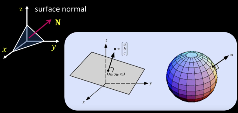
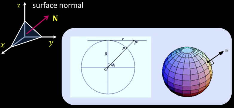
Surface Normals Math

• Let's assume we have a surface $z(x,y)$
• We can define the following

$\color{blue}{-\frac{\partial z}{\partial x}}$ = $\color{blue}{p}$      $\color{blue}{-\frac{\partial z}{\partial y}}$ = $\color{blue}{q}$

Fig.20

Suppose we have a point on the surface. We can define two tangents:

$\color{blue}{t_x = (1,0,-p)^T}$ and $\color{blue}{t_y = (0,1,-q)^T}$

If we want a unit normal, we take

$\color{blue}{n = \frac{N}{||N||} = \frac{t_x\times t_y}{||t_x\times t_y||}=}$ $\color{blue}{\frac{1}{\sqrt{p^2+q^2+1}}(p,q,1)^T}$

Gaussian Sphere and Gradient Space Projection

Fig.21

import numpy as np

def sample_spherical(npoints, ndim=3):
    vec = np.random.randn(ndim, npoints)
    vec /= np.linalg.norm(vec, axis=0)
    return vec

from matplotlib import pyplot as plt
from mpl_toolkits.mplot3d import axes3d
from matplotlib import cm 
phi = np.linspace(0, np.pi, 40)
theta = np.linspace(0, 2 * np.pi, 40)
x = np.outer(np.sin(theta), np.cos(phi))*2
y = np.outer(np.sin(theta), np.sin(phi))*2
z = np.outer(np.cos(theta), np.ones_like(phi))*2
xi, yi, zi = sample_spherical(500)*2

fig, ax = plt.subplots(1, 1, subplot_kw={'projection':'3d', 'aspect':'equal'})
fig.set_size_inches((20,15))
ax.plot_wireframe(x, y, z,color='k', rstride=1, cstride=1)
ax.scatter(xi, yi, zi, s=100, c='r', zorder=10)

<mpl_toolkits.mplot3d.art3d.Path3DCollection at 0x132940be0>

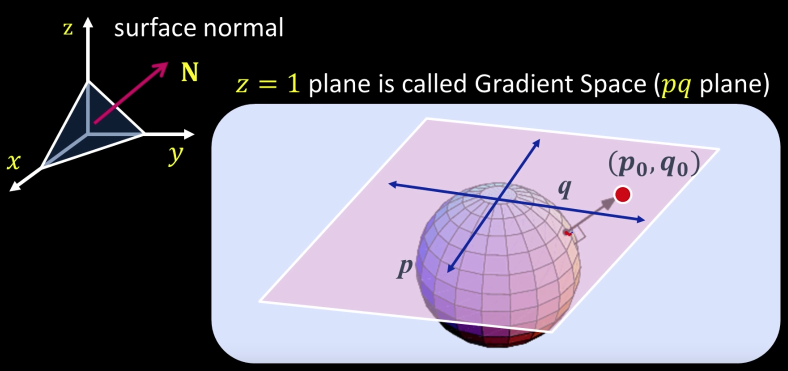
Gradient Space of Source and Normal

Fig.22

Unit normal vector:

$n = \frac{N}{|N|} = \frac{(p,q,1)}{\sqrt{p^2+q^2+1}}$
Unit source vector:

$s = \frac{S}{|S|} = \frac{(p_S,q_S,1)}{\sqrt{p_S^2+q_S^2+1}}$

$$cos\theta_i = n\cdot s = \frac{(pp_s+qq_s+1)}{\sqrt{p^2+q^2+1}\sqrt{p_S^2+q_S^2+1}}$$

%matplotlib inline
fig, ax = plt.subplots(1, 1, subplot_kw={'projection':'3d', 'aspect':'equal'})
fig.set_size_inches((20,15))
ax.plot_wireframe(x, y, z,color='k', rstride=1, cstride=1)
from mpl_toolkits.mplot3d.art3d import Poly3DCollection
xt = [0,1,1]
yt = [0,0,1]
zt = [0,1,0]

p1,p2,p3 = list(zip(xt, yt,zt))
p1,p2,p3 = np.array(p1),np.array(p2),np.array(p3)
u = p2-p1
v = p3-p1
tv = [u[1]*v[2] - u[2]*v[1],
      u[2]*v[0] - u[0]*v[2],u[0]*v[1] - u[1]*v[0]]

## Triangle
verts = [[x1,x2,x3]]
ax.add_collection3d(Poly3DCollection(verts))

## Light
lx=-2;ly=-2;lz=2
ax.scatter([lx],[ly],[lz],s=500, c='y', marker='o')

## Center
ax.scatter([0],[0],[0],s=500, c='r', marker='o')

## Triangle Normal
ax.scatter(tv[0],tv[1],tv[2],s=500, c='b', marker='o')
ax.plot([0,tv[0]],[0,tv[1]],[0,tv[2]],linewidth=7.0)

##Light Normal
lv = np.array([lx,ly,1])/np.sqrt(lx**2+ly**2+1)
ax.scatter(lv[0],lv[1],lv[2],s=500, c='y', marker='o')
ax.plot([0,lv[0]],[0,lv[1]],[0,lv[2]],linewidth=7.0,c='y')

print("The cos(theta): ",np.dot(tv,lv))

The cos(theta):  0.3333333333333333

Shape from Shading Input and Output

Fig.23

Lambertian Case

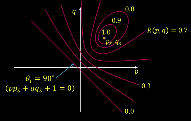
Reflectance map

Relates image brightness $I(x,y)$ to surface orientation $(p,q)$ for given source direction and surface reflectance

Lambertian case

Term:

• K: source brightness
• $\rho$: surface albedo (reflectance)

Image brighness:

• $\color{blue}{I = \rho \cdot k \cdot cos\theta_i = \rho \cdot k(n\cdot s)}$
  let $\color{blue}{\rho \cdot k = 1}$ then $\color{blue}{I = cos\theta_i = n\cdot s}$

Fig.24(a) Lambertian Case

$$\color{blue}{I = cos\theta_i = n \cdot s = \frac{pp_S + qq_S + 1}{\sqrt{p^2 + q^2 + 1}\sqrt{p_S^2+q_S^2+1}} =R(p,q)}$$

$R(p,q)$: Reflectance Map (Lambertian)

Fig.24(b) Lambertian Case

Iso-brightness contours

Fig.25 iso brightness as cos$\theta_i$ changes

import matplotlib.pyplot as plt
import numpy as np

delta = 0.1
xrange = np.arange(-10, 5, delta)
yrange = np.arange(-10, 5, delta)
xs,ys = 1,1
X, Y = np.meshgrid(xrange,yrange)
XS, YS = np.ones(X.shape)*xs,np.ones(X.shape)*ys
# F is one side of the equation, G is the other
F = (X*XS + Y*YS + 1)/(np.sqrt(X**2 + Y**2 + 1)*np.sqrt(XS**2+YS**2+1))
print(Y.shape)
plt.xlim((-1,6))
plt.ylim((-1,6))
for i in np.arange(0,1,0.1):
    plt.contour(X,Y,F, [i])
# plt.contour(X,Y,F, [0.8])
# plt.contour(X,Y,F, [0.7])
# plt.contour(X,Y,F, [0.6])
plt.scatter(xs,ys)
plt.show()

(150, 150)

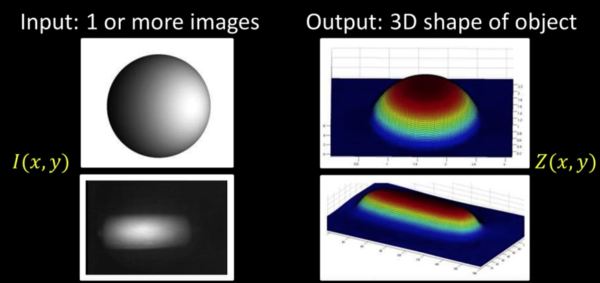
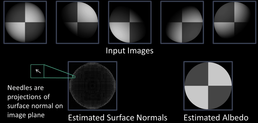
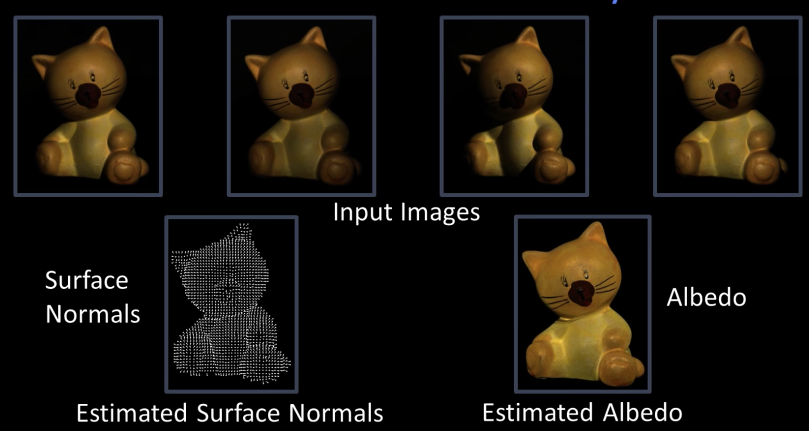
Photometric Stereo

Synthetic results

Fig.26(a)

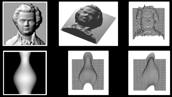
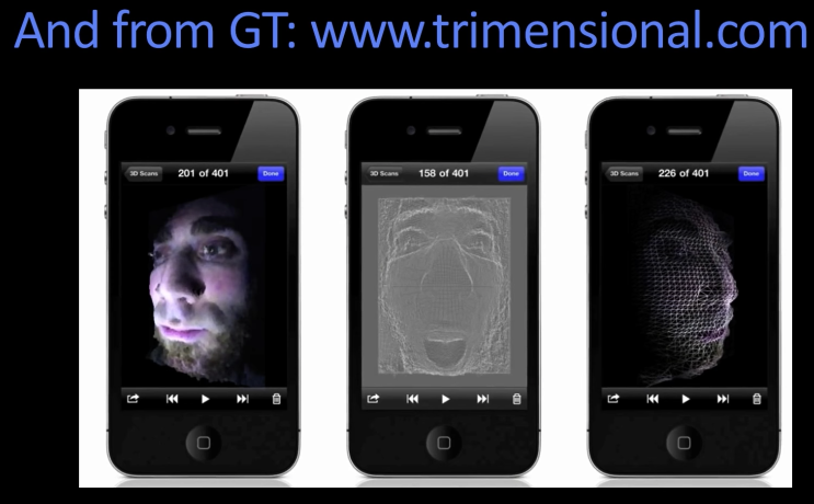
Shape from Shading: "Real" Results

Fig.26(b)

• These single image methods work poorly in practice
• Why? The assumptions are quite restrictive

Need more information:

• Add more constraints: Shape-from-shading
• Take more images: Photometric stereo

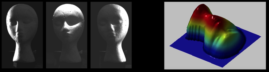
Photometric stereo

Input: Several images

• Same object
• Different lightings
• Sampe pose

output

• 3D shape of object
• Albedo at $(x,y)$

Fig.26(c)

Solving the Equations

Photmetric stereo

Image brightness:

$$\color{blue}{I = \rho \cdot k \cdot cos\theta_i = \rho n \cdot s}$$

Where $(k = 1)$

$$\color{blue}{I_1 = \rho n \cdot s_1}$$ $$\color{blue}{I_2 = \rho n \cdot s_2}$$ $$\color{blue}{I_3 = \rho n \cdot s_3}$$

Write this as a matrix equation:

$$\color{blue}{\begin{bmatrix}I_1\\ I_2\\ I_2\end{bmatrix} = \rho \begin{bmatrix}S_1^T\\ S_2^T\\ S_2^T\end{bmatrix}n}$$

Fig.27

$\color{blue}{I}$ and $\color{blue}{S}$ are known
$$\color{blue}{\rho n = \tilde{n}}$$ $$\color{blue}{\tilde{n} = S^{-1} I}$$ $$\color{blue}{\rho = |\tilde{n}|}$$ $$\color{blue}{n = \frac{\tilde{n}}{|\tilde{n}|}=\frac{\tilde{n}}{\rho}}$$

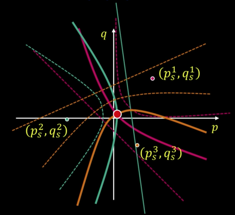
Adding more light sources

Get better results by using more ($M$) lights:

$$\color{blue}{\begin{bmatrix}I_1\\ . \\. \\. \\ I_M\end{bmatrix} = \begin{bmatrix}S_1^T\\ . \\. \\. \\ S_M^T\end{bmatrix}\rho n}$$

Least squares solutions

$$\color{blue}{I = S\tilde{n}}$$

$\color{blue}{M \times 1 = (M \times 3)(3\times1)}$ $$\color{blue}{S^TI = S^TS\tilde{n}}$$ $$\color{blue}{\tilde{n} = (S^TS^{-1})S^TI}$$

Moore-Penrose pseudo inverse $\color{blue}{min||I-S\tilde{n}||_2^2}$

pq Space

Photometric stereo: pq space

Fig.28

import matplotlib.pyplot as plt
import numpy as np

def contour(xs,ys,ax):
    delta = 0.1
    xrange = np.arange(-10, 5, delta)
    yrange = np.arange(-10, 5, delta)
    X, Y = np.meshgrid(xrange,yrange)
    XS, YS = np.ones(X.shape)*xs,np.ones(X.shape)*ys
    # F is one side of the equation, G is the other
    F = (X*XS + Y*YS + 1)/(np.sqrt(X**2 + Y**2 + 1)*np.sqrt(XS**2+YS**2+1))
    print(Y.shape)
    plt.xlim((-6,6))
    plt.ylim((-6,6))
    for i in np.arange(0,1,0.1):
        ax.contour(X,Y,F, [i])
    ax.scatter(xs,ys)
    
    
ax = plt.gca()
contour(1,1,ax)
contour(-1,-1,ax)
contour(-1,1,ax)
plt.show()

(150, 150)
(150, 150)
(150, 150)

Examples

Results: Lambertian sphere

Fig.29 (a)

Fig.29 (b)

Fig.29 (c) www.trimensional.com

Real Application

Fig.30(a)

Human shape from shading

Fig.30(b)

Also check Ramachandran's work on Shape from Shading by Humans

http://psy.ucsd.edu/chip/ramabio.html

Messi On Contours

## from https://stackoverflow.com/questions/41624616/plot-implicit-equations-in-python-3

import matplotlib.pyplot as plt
import numpy as np
messi400 = imread("imgs/messi400.jpg")
delta = 0.1
xrange = np.arange(-10, 10, delta)
yrange = np.arange(-10, 10, delta)
X, Y = np.meshgrid(xrange,yrange)
messi_heart = np.ones(messi400.shape).astype(np.int)*255
# F is one side of the equation, G is the other
F = X**2
G = 1 - (1.08*Y/1.1 - np.sqrt(np.abs(X)))**2
print(F.shape,G.shape)

plt.gca().imshow(np.flipud(gray(messi400[90:290,160:360])),origin='lower')
Z = F-G
Z[X<-10] = None
Z[X>10] = None
x = plt.contour(Z, [50],colors="red",
                levels=np.arange(50, 220, 20))

plt.show()

(200, 200) (200, 200)

Cannot believe this guy. I just bought the ticket for Lyon vs Barca in Lyon on Feb 19th. I am flying to Lyon on the 18th. I wish he spreads his magic all over my eyes in reality as he has been doing through my curved Samsung screen