

Image Point Matching Problem
- Suppose I have two images related by some transformation Or have two images of the same object in different positions.
- How to find the transformation of image 1 that would align it with image 2
We want Local$ ^{(1)}$ Features$ ^{(2)}$
Not machine learning features, but things that we compute about little region or spots
- Goal: Find point in an image that can be:
- Found in other images
- Found precisely - well localized
- Found reliably - well matched
Why?
- Want to compute a fundamental matrix to recover geometry
- Robotics/vision: See how a bunch of points move from one frame to another. Allows computation of how camera moved -> depth -> moving objects
- Build a panorama

Matching with Features
- Detect features (features points) in both images
- Match features - find corresponding pairs
- Use these pairs to align images

- Problem 1:
- Detec the same point independently in both

Fig.2 (c): No chance to match
- Detec the same point independently in both
- Problem 2:
- For each point correctly recognize the corresponding one
Fig.2 (d): Which point is which
- For each point correctly recognize the corresponding one
More motivation...
- Feature points are used also for:
- Image alignment (e.g. homography or fundamental matrix)
- 3D reconstruction
- Mortion tracking
- Object recognition
- Indexing and database retrieval
- Robot navigation
- ... Other
**Quize**

Characteristics of Good Features
Repeatability/Precision
- The same feature can be found in several images despite geometric and photometric transformation
Saliency/Matchability
- Each feature has a distinctive description
Compactness and efficiency
- Many fewer features than image pixels
Locality
- A feature occupies a relatively small area of the image; robust to clutter and occlusion
In [9]:
import numpy as np
import cv2
from matplotlib import pyplot as plt
import PIL
from io import BytesIO
from IPython.display import clear_output, Image as NoteImage, display
def imshow(im,fmt='jpeg'):
#a = np.uint8(np.clip(im, 0, 255))
f = BytesIO()
PIL.Image.fromarray(im).save(f, fmt)
display(NoteImage(data=f.getvalue()))
def imread(filename):
img = cv2.imread(filename)
img = cv2.cvtColor(img, cv2.COLOR_BGR2RGB)
return img
def red(im):
return im[:,:,0]
def green(im):
return im[:,:,1]
def blue(im):
return im[:,:,2]
def gray(im):
return cv2.cvtColor(im, cv2.COLOR_BGR2GRAY)
def square(img,center,size,color=(0,255,0)):
y,x = center
leftUpCorner = (x-size,y-size)
rightDownCorner = (x+size,y+size)
cv2.rectangle(img,leftUpCorner,rightDownCorner,color,3)
def normalize_img(s):
start = 0
end = 255
width = end - start
res = (s - s.min())/(s.max() - s.min()) * width + start
return res.astype(np.uint8)
def line(img,x):
cv2.line(img,(0,x),(img.shape[1],x),(255,0,0),3)
def mse(imageA, imageB):
# the 'Mean Squared Error' between the two images is the
# sum of the squared difference between the two images;
# NOTE: the two images must have the same dimension
err = np.sum((imageA.astype("float") - imageB.astype("float")) ** 2)
err /= float(imageA.shape[0] * imageA.shape[1])
# return the MSE, the lower the error, the more "similar"
# the two images are
return err
def random_color():
color = list(np.random.choice(range(256), size=3))
return (int(color[0]),int(color[1]),int(color[2]))
In [2]:
import numpy as np
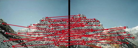
img1 = imread('imgs/left.jpg') #queryimage # left image
img2 = imread('imgs/right.jpg') #trainimage # right image
gimg1=red(img1)
gimg2=red(img2)
sift = cv2.xfeatures2d.SIFT_create()
# find the keypoints and descriptors with SIFT
kp1, des1 = sift.detectAndCompute(gimg1,None)
kp2, des2 = sift.detectAndCompute(gimg2,None)
# FLANN parameters
FLANN_INDEX_KDTREE = 0
index_params = dict(algorithm = FLANN_INDEX_KDTREE, trees = 5)
search_params = dict(checks=50)
flann = cv2.FlannBasedMatcher(index_params,search_params)
matches = flann.knnMatch(des1,des2,k=2)
good = []
pts1 = []
pts2 = []
# ratio test as per Lowe's paper
for i,(m,n) in enumerate(matches):
if m.distance < 0.8*n.distance:
good.append(m)
pts2.append(kp2[m.trainIdx].pt)
pts1.append(kp1[m.queryIdx].pt)
pts1 = np.int32(pts1)
pts2 = np.int32(pts2)
F, mask = cv2.findFundamentalMat(pts1,pts2,cv2.FM_LMEDS)
# We select only inlier points
pts1 = pts1[mask.ravel()==1]
pts2 = pts2[mask.ravel()==1]
for p1,p2 in zip(pts1,pts2):
c = random_color()
cv2.circle(img1,(int(p1[0]),int(p1[1])),10,c,-11)
cv2.circle(img2,(int(p2[0]),int(p2[1])),10,c,-11)
# img3,img4 = drawlines(img2,img1,lines2,pts2,pts1)
fig = plt.gcf()
fig.set_size_inches((20,15))
plt.subplot(121),plt.imshow(img1)
plt.subplot(122),plt.imshow(img2)
plt.show()

Haris Corners
Mathematics
Change in appearance for the shift [u,v]:
$$\color{blue}{E(u,v)=\sum_{x,y}w(x,y)[I(x + u,y+v)-I(x,y)]^2}$$
$\color{blue}{I}$: Intensity image $\color{blue}{u,v}$: are small shifts $\color{blue}{w}$: window function
Window function w(x,y) can be 1 in window, 0 outside or Gaussian
In [3]:
from scipy import signal
from scipy.fftpack import fft, fftshift
import matplotlib.pyplot as plt
window = signal.gaussian(51, std=7)
ax1 = plt.subplot(211)
ax1.plot(window)
ax1.set_title(r"Gaussian window ($\sigma$=7)")
ax1.set_ylabel("Amplitude")
ax1.set_xlabel("Sample")
window = signal.tukey(51)
ax2 = plt.subplot(212)
ax2.plot(window)
ax2.set_title("Tukey window")
ax2.set_ylabel("Amplitude")
ax2.set_xlabel("Sample")
ax2.set_ylim([0, 1.1])
fig = plt.gcf()
fig.set_size_inches((10,10))

In [4]:
filename = 'imgs/chess.jpg'
img = imread(filename)
gimg = gray(img)
gimg = np.float32(gimg)
dst = cv2.cornerHarris(gimg,2,3,0.04)
#result is dilated for marking the corners, not important
dst = cv2.dilate(dst,None)
# Threshold for an optimal value, it may vary depending on the image.
img[dst>0.01*dst.max()]=[0,0,255]
imshow(img)

🤴 Lets try it on the King Messi 🤴
In [80]:
def calculate_haris_corner(img,show=True):
if type(img) == str:
img = imread(img)
gimg = gray(img)
gimg = np.float32(gimg)
dst = cv2.cornerHarris(gimg,2,3,0.04)
#result is dilated for marking the corners, not important
dst = cv2.dilate(dst,None)
# Threshold for an optimal value, it may vary depending on the image.
img[dst>0.01*dst.max()]=[0,0,255]
if show:
imshow(img)
return np.argwhere(dst>0.01*dst.max())
In [69]:
calculate_haris_corner("imgs/messi.jpg")

Out[69]:
In [7]:
calculate_haris_corner("imgs/messi4.jpg")

Out[7]:
In [8]:
calculate_haris_corner("imgs/messi_alaves.jpg")

Out[8]:
In [9]:
calculate_haris_corner("imgs/messi_espanyol.jpg")

Out[9]:
👑2 days ago, Lionel Messi scored two direct free-kicks in a single La Liga game for the first time as Barcelona beat Espanyol to move three points clear at the top.👑
Small Shifts
$$\color{blue}{E(u,v)=\sum_{x,y}w(x,y)[I(x + u,y+v)-I(x,y)]^2}$$
We want to find out how the error/energy function behaves for small shifts (u,v near 0,0)
We are going to do second-order Taylor expansion of E(u,v) about (0,0) (local quadratic approximation for small (u,v)
$$\color{blue}{F(\delta x) \approx F(0) + \delta x \cdot \frac{dF(0)}{dx} + \frac{1}{2}\delta x^2\cdot\frac{d^2F(0)}{dx^2}}$$
$$\color{blue}{E(u,v) \approx E(0,0) + \begin{bmatrix}u&v\end{bmatrix} \begin{bmatrix}E_u(0,0)\\E_v(0,0)\end{bmatrix} + \frac{1}{2}\begin{bmatrix}u&v\end{bmatrix}\begin{bmatrix}E_{uu}(0,0) & E_{uv}(0,0)\\E_{uv}(0,0)&E_{vv}(0,0)\end{bmatrix} \begin{bmatrix}u \\ v\end{bmatrix} }$$
Second- Order Taylor Expansion
Second-order Taylor expansion of E(u,v) about (0,0)
$$\color{blue}{E_u(u,v) = \sum_{x,y}2w(x,y)[I(x+u,y+v)-I(x,y)]I_x(x+u,y+v)}$$
u: is the offset in the x direction
$$\color{blue}{E_{uu}(u,v) = \sum_{x,y}2w(x,y)I_x(x+u,y+v)I_x(x+u,y+v) + \sum_{x,y}2w(x,y)[I(x+u,y+v)-I(x,y)]I_{xx}(x+u,y+v)}$$
$$\color{blue}{E_{uv}(u,v) = \sum_{x,y}2w(x,y)I_y(x+u,y+v)I_x(x+u,y+v) + \sum_{x,y}2w(x,y)[I(x+u,y+v)-I(x,y)]I_{xy}(x+u,y+v)}$$
Evalute E and its deivatives at (0,0)
$$\color{blue}{E(u,v) \approx E(0,0) + \begin{bmatrix}u&v\end{bmatrix} \begin{bmatrix}E_u(0,0)\\E_v(0,0)\end{bmatrix} + \frac{1}{2}\begin{bmatrix}u&v\end{bmatrix}\begin{bmatrix}E_{uu}(0,0) & E_{uv}(0,0)\\E_{uv}(0,0)&E_{vv}(0,0)\end{bmatrix} \begin{bmatrix}u \\ v\end{bmatrix} }$$
$$\color{blue}{E_u(0,0) = \sum_{x,y}2w(x,y)[I(x,y)-I(x,y)]I_x(x,y)}$$
$$\color{blue}{E_{uu}(0,0) = \sum_{x,y}2w(x,y)I_x(x,y)I_x(x,y) + \sum_{x,y}2w(x,y)[I(x,y)-I(x,y)]I_{xx}(x,y)}$$
$$\color{blue}{E_{uv}(0,0) = \sum_{x,y}2w(x,y)I_y(x,y)I_x(x,y) + \sum_{x,y}2w(x,y)[I(x,y)-I(x,y)]I_{xy}(x,y)}$$
$\implies$
$$\color{blue}{E(u,v) \approx E(0,0) + \begin{bmatrix}u&v\end{bmatrix} \begin{bmatrix}E_u(0,0)\\E_v(0,0)\end{bmatrix} + \frac{1}{2}\begin{bmatrix}u&v\end{bmatrix}\begin{bmatrix}E_{uu}(0,0) & E_{uv}(0,0)\\E_{uv}(0,0)&E_{vv}(0,0)\end{bmatrix} \begin{bmatrix}u \\ v\end{bmatrix} }$$
$$\color{blue}{E(0,0) = 0}$$ $$\color{blue}{E_u(0,0) = 0}$$ $$\color{blue}{E_v(0,0) = 0}$$
$$\color{blue}{E_{uu}(0,0) = \sum_{x,y}2w(x,y)I_x(x,y)I_x(x,y)}$$ $$\color{blue}{E_{vv}(0,0) = \sum_{x,y}2w(x,y)I_y(x,y)I_y(x,y)}$$ $$\color{blue}{E_{uv}(0,0) = \sum_{x,y}2w(x,y)I_x(x,y)I_y(x,y)}$$
$\implies$
$$\color{blue}{E(u,v) \approx \begin{bmatrix}u&v\end{bmatrix} \begin{bmatrix}\sum_{x,y}w(x,y)I^2_x(x,y) & \sum_{x,y}w(x,y)I_x(x,y)I_y(x,y) \\ \sum_{x,y}w(x,y)I_x(x,y)I_y(x,y) & \sum_{x,y}w(x,y)I^2_y(x,y)\end{bmatrix} \begin{bmatrix}u \\ v\end{bmatrix}}$$
Quadratic Approximation Simlification
The quadratic approximation simplifies to $$\color{blue}{E(u,v) \approx \begin{bmatrix}u&v\end{bmatrix}M\begin{bmatrix}u \\ v\end{bmatrix}}$$
Where M is the second moment matrix computed from image derivatives
$$\color{blue}{M = \sum_{x,y} w(x,y) \begin{bmatrix}I^2_x & I_xI_y \\ I_xI_y&I^2_y\end{bmatrix}}$$
furthermore, the second moment matrix can be written (without the weight):
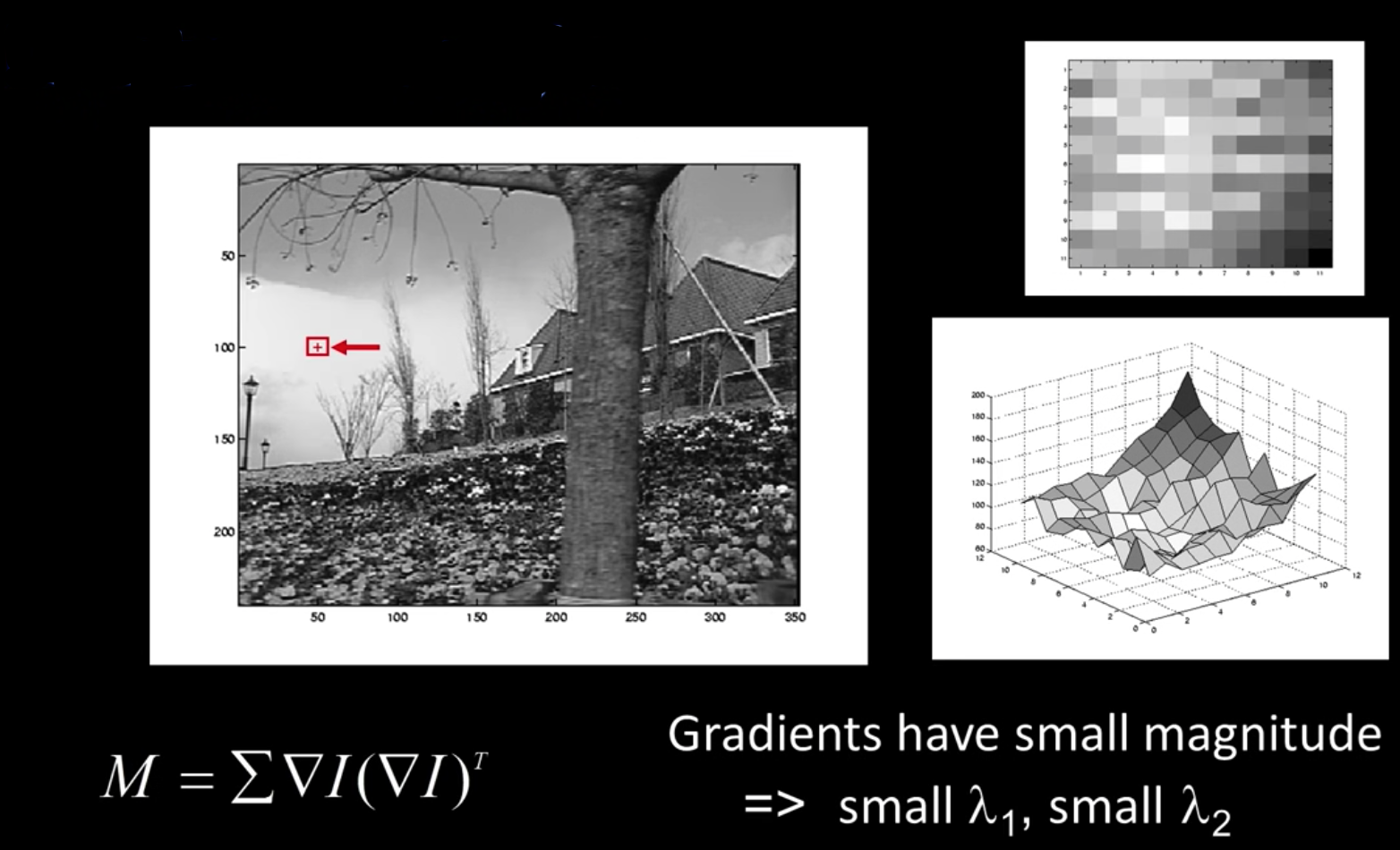
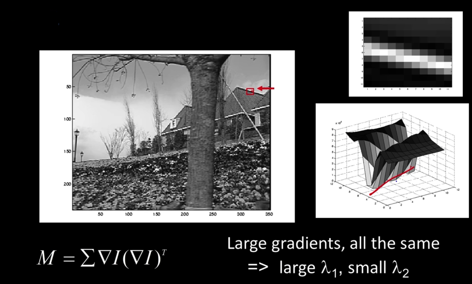
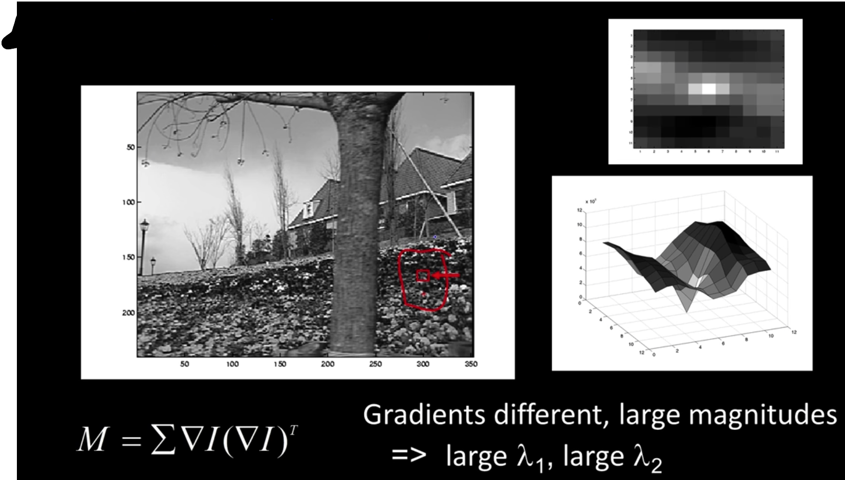
$$\color{blue}{M = \begin{bmatrix} \sum I_xI_x & \sum I_xI_y \\ \sum I_xI_y & \sum I_yI_y\end{bmatrix} = \sum (\begin{bmatrix}I_x \\ I_y\end{bmatrix}\begin{bmatrix}I_x & I_y\end{bmatrix}) = \sum \nabla I(\nabla I)^T}$$
Interpreting the Second Moment Matrix
The surface E(u,v) is locally approximated by a quadratic form
$$\color{blue}{E(u,v) \approx \begin{bmatrix}u&v\end{bmatrix}M\begin{bmatrix}u \\ v\end{bmatrix}}$$
$$\color{blue}{M = \sum_{x,y} w(x,y) \begin{bmatrix}I^2_x & I_xI_y \\ I_xI_y&I^2_y\end{bmatrix}}$$

Consider a constant "slice" of E(u,v):
$$\color{blue}{\sum I^2_xu^2 + 2\sum I_xI_yuv + \sum I^2_yv^2 = k}$$
$$\color{blue}{\begin{bmatrix}u&v\end{bmatrix}M\begin{bmatrix}u \\ v\end{bmatrix} = const}$$
The first equation is an equation of an eliplse in the (u,v) space

First, consider the axis-aligned case where gradients are either horizontal or vertical
$$\color{blue}{M = \sum_{x,y} w(x,y) \begin{bmatrix}I^2_x & I_xI_y \\ I_xI_y&I^2_y\end{bmatrix} = \begin{bmatrix}\lambda_1& 0 \\ 0&\lambda_2\end{bmatrix}}$$
If either $\color{blue}{\lambda}$ is close to 0, then this is not a corner, so look for locations where both are large
Diagonalization of M: $\color{blue}{M = R^{-1}\begin{bmatrix}\lambda_1& 0 \\ 0&\lambda_2\end{bmatrix}R}$
The axis lengths of the ellipse are determined by the eigenvalues and the orientation is determined by R

Interpreting the eigenvalues
Classification of image points using eignvalues of $\color{blue}{M}$:

Harris Corner Response Function
$$\color{blue}{R = det(M) - \alpha trace(M)^2 = \lambda_1\lambda_2 - \alpha(\lambda_1 + \lambda_2)^2}$$
$\color{blue}{\alpha}$: constant (0.04 to 0.06)

R depends only on eigenvalues of M, but don't compute them (no sqrt, so really fast even in the '80s)
R is large for a corner
R is negative with large magnitued for an edge
|R| is small a flat region
In [11]:
import numpy as np
import cv2 as cv
from matplotlib import pyplot as plt
img = imread('imgs/nature.jpg')
gimg = green(img)
laplacian = cv.Laplacian(gimg,cv.CV_64F)
sobelx = cv.Sobel(gimg,cv.CV_64F,1,0,ksize=5)
sobely = cv.Sobel(gimg,cv.CV_64F,0,1,ksize=5)
plt.subplot(2,2,1),plt.imshow(gimg,cmap = 'gray')
plt.title('Original'), plt.xticks([]), plt.yticks([])
plt.subplot(2,2,2),plt.imshow(laplacian,cmap = 'gray')
plt.title('Laplacian'), plt.xticks([]), plt.yticks([])
plt.subplot(2,2,3),plt.imshow(sobelx,cmap = 'gray')
plt.title('Sobel X'), plt.xticks([]), plt.yticks([])
plt.subplot(2,2,4),plt.imshow(sobely,cmap = 'gray')
plt.title('Sobel Y'), plt.xticks([]), plt.yticks([])
fig = plt.gcf()
fig.set_size_inches((10,10))

In [11]:
water = gimg[330:380,200:250]
wateredge = gimg[260:310,500:550]
summit = gimg[60:110,320:370]
gwater = cv.Laplacian(water,cv.CV_64F)
gwateredge = cv.Laplacian(wateredge,cv.CV_64F)
gsummit = cv.Laplacian(summit,cv.CV_64F)
plt.subplot(3,2,1),plt.imshow(water,cmap = 'gray')
plt.title('Low Texture Region'), plt.xticks([]), plt.yticks([])
plt.subplot(3,2,2),plt.imshow(gwater,cmap = 'gray')
plt.title('Gradient'), plt.xticks([]), plt.yticks([])
plt.subplot(3,2,3),plt.imshow(wateredge,cmap = 'gray')
plt.title('Edge'), plt.xticks([]), plt.yticks([])
plt.subplot(3,2,4),plt.imshow(gwateredge,cmap = 'gray')
plt.title('Gradient'), plt.xticks([]), plt.yticks([])
plt.subplot(3,2,5),plt.imshow(summit,cmap = 'gray')
plt.title('Corner'), plt.xticks([]), plt.yticks([])
plt.subplot(3,2,6),plt.imshow(gsummit,cmap = 'gray')
plt.title('Gradient'), plt.xticks([]), plt.yticks([])
fig = plt.gcf()
fig.set_size_inches((10,10))

Harris detector: Algorithm
- Compute Gaussian derivatives at each pixel
- Compute second moment matrix M in a Gaussian window around each pixel
- Compute corner response function R
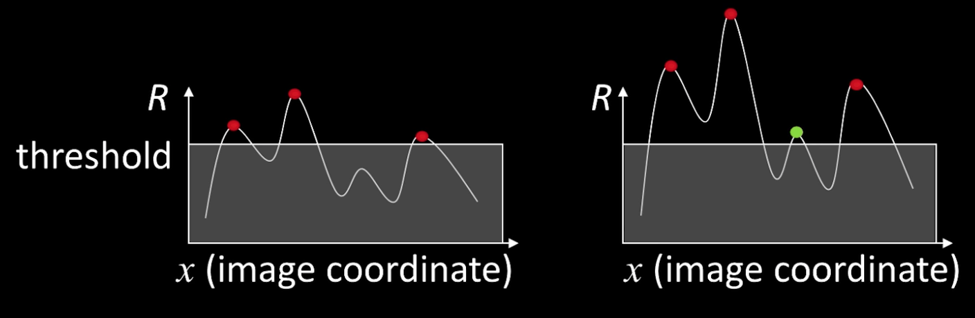
- Threshold R
- Find local maxima of response function (nonmaximum suppression)
Harris Detector Workflow


In [12]:
def findCorners(filename, window_size, k, thresh):
"""
Finds and returns list of corners and new image with corners drawn
:param img: The original image
:param window_size: The size (side length) of the sliding window
:param k: Harris corner constant. Usually 0.04 - 0.06
:param thresh: The threshold above which a corner is counted
:return:
"""
img = imread(filename)
gimg = gray(img)
#Find x and y derivatives
dx = cv.Sobel(gimg,cv.CV_64F,1,0,ksize=5)
dy = cv.Sobel(gimg,cv.CV_64F,0,1,ksize=5)
Ixx = dx**2
Ixy = dy*dx
Iyy = dy**2
height = int(img.shape[0])
width = int(img.shape[1])
cornerList = []
color_img = img.copy()
offset = int(window_size/2)
#Loop through image and find our corners
for y in range(offset, height-offset):
for x in range(offset, width-offset):
#Calculate sum of squares
windowIxx = Ixx[y-offset:y+offset+1, x-offset:x+offset+1]
windowIxy = Ixy[y-offset:y+offset+1, x-offset:x+offset+1]
windowIyy = Iyy[y-offset:y+offset+1, x-offset:x+offset+1]
Sxx = windowIxx.sum()
Sxy = windowIxy.sum()
Syy = windowIyy.sum()
#Find determinant and trace, use to get corner response
det = (Sxx * Syy) - (Sxy**2)
trace = Sxx + Syy
r = det - k*(trace**2)
## For some reason the values are very high, so devide
r = r/1000000000000.0
#If corner response is over threshold, color the point and add to corner list
if r > thresh:
cornerList.append([x, y, r])
color_img.itemset((y, x, 0), 0)
color_img.itemset((y, x, 1), 0)
color_img.itemset((y, x, 2), 255)
imshow(color_img)
In [13]:
print("OpenCV implementation")
calculate_haris_corner('imgs/nature.jpg')
print("Local implementation")
findCorners("imgs/nature.jpg",2.0,0.04,10.0)


Other corners:
Shi-Tomasi '94:
"Cornerness" = $\color{blue}{min(\lambda_1,\lambda_2)}$ Find local maximums cvGoodFeaturesToTrack(..)
Reportedly better for refion undergoing affine deformations
Brown, M., Szeliski, R., and Winder, S. (2005): $$\color{blue}{\frac{det\,\, M}{tr\,\, M} = \frac{\lambda_0\lambda_1}{\lambda_0+\lambda_1}}$$
There are others....
In [1]:
## cvGoodFeaturesToTrack
Harris Detector Properties
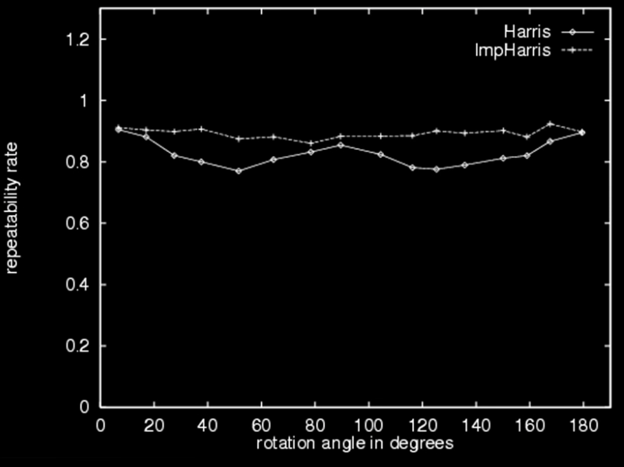
Rotation invariance?
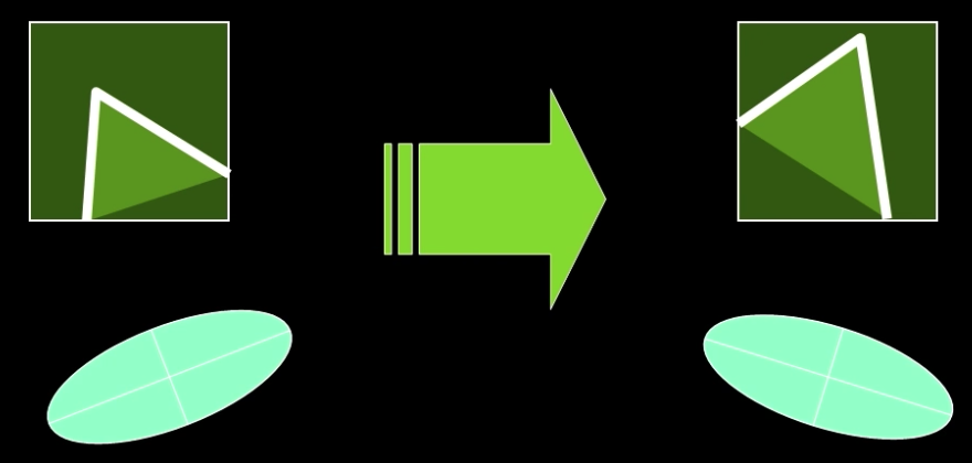
Ellipse rotates but its shape (i.e. eigenvalues) remains the same
Repeatability rate:
$$\color{blue}{\frac{\# correspondences}{\# possible\,\, correspondences}}$$
In [2]:
## You are welcome to show the previous theory in code....
More Haris Detector Properties
- Mostly invariant to additive and multiplicative intensity changes(threshold issue for multiplicative)
- Only derivatives are used -> invariance to intensity shift $\color{blue}{I \rightarrow I + b}$
- Intensity scale: $\color{blue}{I \rightarrow a*I}$
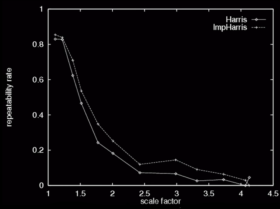
- Invariant to image scale?
- Not invariant to image scale!

In [3]:
## You are welcome to show the previous theory in code....
Scale Invariant Detection
- Consider regions (e.g. circles) of different sizes around a point
Regions of corresponding sizes will look the same in both images
The problem: how do we choose corresponding circles independently in each image?
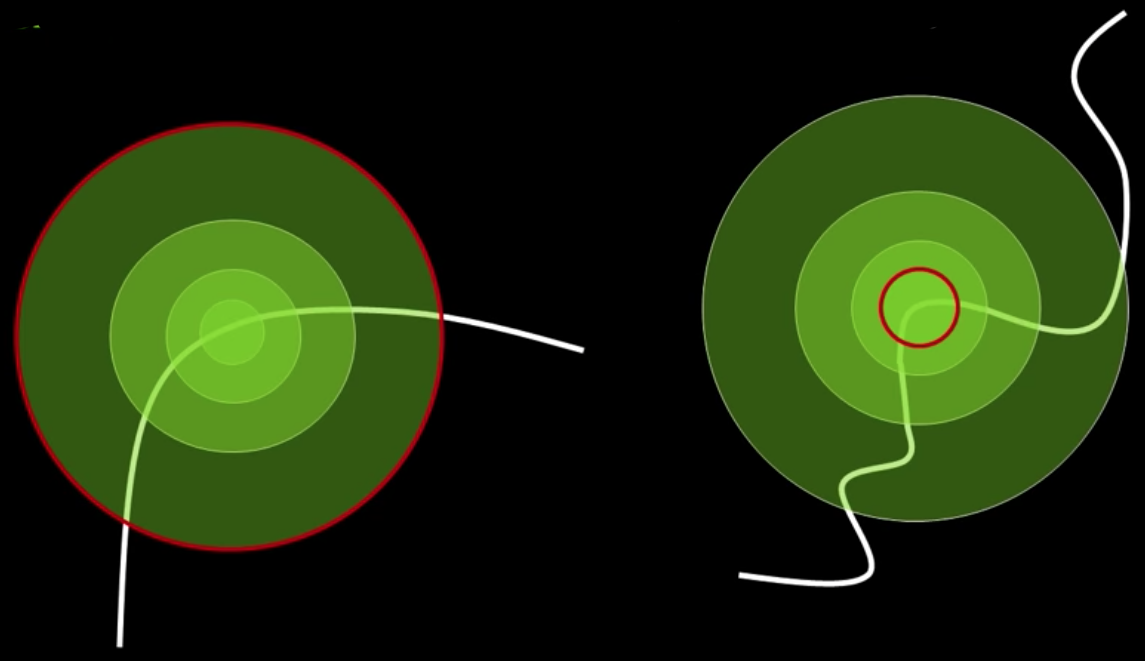
Solution:
Design a function on the region (circle), which is "scale invariant" - not affected by the size but will be the same for "corresponding regions," even if they are at different sizes/scales
Example: Average intensity. For corresponding regions (even of different sizes) it will be the same
One Method fro Scale Invariant Detection
One method:
- At a point, compute the scale invariant function of different size neighborhoods (different scales).
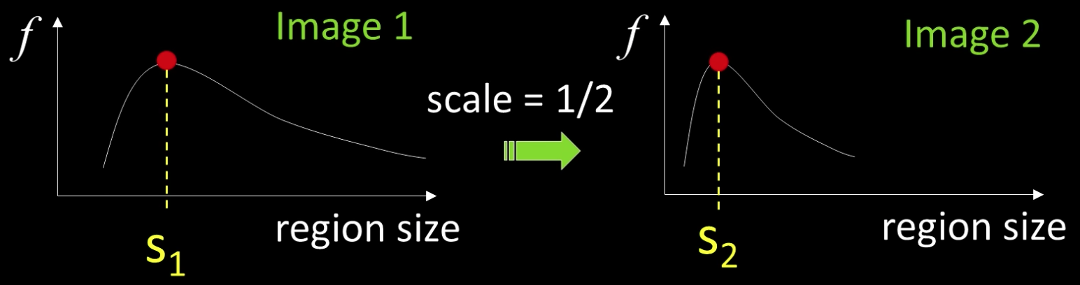
- Important: this scale invariant region size is found in each image independently
In [4]:
## You are welcome to show the previous theory in code....
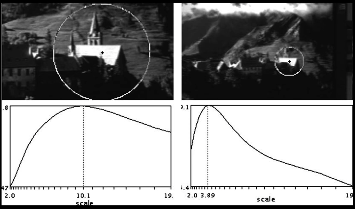
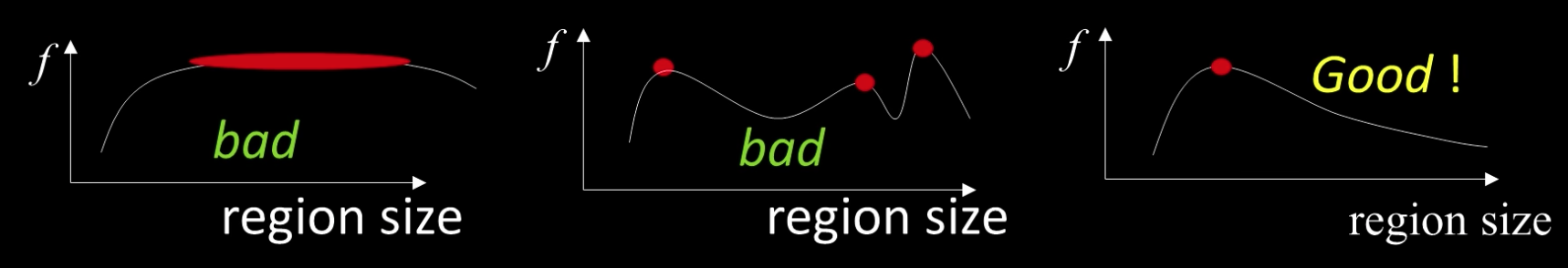
A Food Function for Scale Detection
- A "good" function for scale detection: has one stable sharp peak
For usual images: a good function would be a one which responds to contrast (sharp local intensity change)
Function is just application of a kernel: f = Kernel * Image
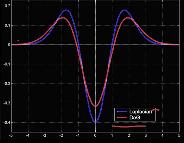
$$\color{blue}{ L = \sigma^2(G_{xx}(x,y,\sigma) + G_{yy}(x,y,\sigma))}$$
Laplacian of Gaussian- LoG
$$\color{blue}{ DoG = \sigma^2(G_{xx}(x,y,k\sigma) + G_{yy}(x,y,\sigma))}$$
Difference of Gaussians
Both kernals are invariant to scale and rotation
In [18]:
## Show Laplacian of Gaussian
from mpl_toolkits.mplot3d import Axes3D
import matplotlib.pyplot as plt
from matplotlib import cm
from matplotlib.ticker import LinearLocator, FormatStrFormatter
import numpy as np
fig = plt.figure()
ax = fig.gca(projection='3d')
# Make data.
X = np.arange(-5, 5, 0.25)
Y = np.arange(-5, 5, 0.25)
X, Y = np.meshgrid(X, Y)
#R = np.sqrt(X**2 + Y**2)
#R = X**2 + Y**2
sigma = 2
Z = -1*1/(np.pi*np.power(sigma,4))*(1-(X**2 + Y**2)/(2*np.power(sigma,2)))*np.exp(-(X**2 + Y**2)/(2*np.power(sigma,2)))
Z *= -1
# Plot the surface.
surf = ax.plot_surface(X, Y, Z, cmap=cm.coolwarm,
linewidth=0, antialiased=False)
# Customize the z axis.
ax.zaxis.set_major_locator(LinearLocator(10))
ax.zaxis.set_major_formatter(FormatStrFormatter('%.02f'))
# Add a color bar which maps values to colors.
fig.colorbar(surf, shrink=0.5, aspect=5)
plt.show()

In [19]:
from scipy import ndimage, misc
import matplotlib.pyplot as plt
ascent = misc.ascent()
fig = plt.figure()
plt.gray() # show the filtered result in grayscale
ax1 = fig.add_subplot(121) # left side
ax2 = fig.add_subplot(122) # right side
result = ndimage.gaussian_laplace(ascent, sigma=1)
ax1.imshow(result)
result = ndimage.gaussian_laplace(ascent, sigma=3)
ax2.imshow(result)
plt.show()

Key Point Localization
- General idea: find robust extremum (maximum of minimum) both in space in scale
- Specific suggestion: use DoG pyramid to find maximum values (remember edge detection?) - then eliminate "edges" and pick only corners
Scale space processed one octave at a time

Each point is compared to its 8 neighbors in the current image and 0 neighbors each in the scale above and below

Extrema at different scales


Scale Invariant Detectors
SIFT(LOWE)
Find local maximum of:
- Difference of Gaussians in space and scale

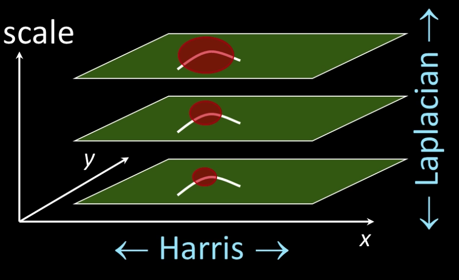
Harris-Laplacian
Find local maximum of:
- Harris corner detector in space (image coordinates)
- Laplacian in scale

In [107]:
## Code to show comparision
import itertools
import cv2
def resize(image,size):
return cv2.resize(image, size)
def get_box(nx,ny,center_x,center_y,size):
x = center_x
y = center_y
x_i = np.arange(max(0,x-size),min(nx,x+size))
y_i = np.arange(max(0,y-size),min(ny,y+size))
return list(itertools.product(x_i,y_i))
def set_corner(img,x,y,size=3,color=[0,0,255]):
box = get_box(img.shape[1],img.shape[0],x,y,size)
for x,y in box:
img.itemset((y, x, 0), color[0])
img.itemset((y, x, 1), color[1])
img.itemset((y, x, 2), color[2])
def calculate_sift_corner(img,show=True,plotid=111):
if type(img) == str:
img = imread(img)
gimg = gray(img)
sift = cv2.xfeatures2d.SIFT_create()
kp = sift.detect(gimg,None)
for p in kp:
#print(x.pt)
x,y = min(int(p.pt[0]),img.shape[1]-1),min(int(p.pt[1]),img.shape[0]-1)
set_corner(img,x,y,2)
if show:
ax = plt.subplot(plotid)
ax.set_title("Sift Corner")
ax.imshow(img)
return kp
def calculate_haris_corner(img,show=True,plotid=111):
if type(img) == str:
img = imread(img)
gimg = gray(img)
gimg = np.float32(gimg)
dst = cv2.cornerHarris(gimg,2,3,0.04)
#result is dilated for marking the corners, not important
dst = cv2.dilate(dst,None)
# Threshold for an optimal value, it may vary depending on the image.
img[dst>0.01*dst.max()]=[0,0,255]
if show:
ax = plt.subplot(plotid)
ax.set_title("Harris Corner")
ax.imshow(img)
return np.argwhere(dst>0.01*dst.max())
nature = imread('imgs/nature.jpg')
nx,ny,_ = nature.shape
# corners_center = [(90,65,3),(185,100,3),(354,82,3),(430,113,3),
# (478,102,3),(354,269,3),(211,245,3),
# (215,302,3),(233,235,3),(160,346,3)]
n = 30
scales = np.linspace(1,0.1,n)
## Harris corners with scale
harris_p = calculate_haris_corner(nature.copy(),plotid=221)
possible = len(harris_p)
harris_per = [len(calculate_haris_corner(resize(nature.copy(),(int(ny*s),int(nx*s))),False))/possible for s in scales]
## Sift corners with scale
sift_p = calculate_sift_corner(nature.copy(),plotid=222)
possible = len(sift_p)
sift_per = [len(calculate_sift_corner(resize(nature.copy(),(int(ny*s),int(nx*s))),False))/possible for s in scales]
ax = plt.subplot(223)
ax.plot(np.arange(n),harris_per,label="Harris")
ax.plot(np.arange(n),sift_per,label="Sift")
ax.legend()
ax.set_title("Repeatability Rate")
fig = plt.gcf()
fig.set_size_inches((20,15))

Point Descriptors
How to match points detected using, for example, Harris detector?
- We need to describe them -a descriptor
Criteria for Point Descriptors
We want the descriptors to be the (almost: without duplication) same in both image - invariant
We also need the descriptors to be distinctive (different points have different descriptors)
Simple solution? Not so good
- Harris gives good detection - and we also know the scale
Why not just use correlation to check the match of the window around the feature in image 1 with every feature in image 2
Not so good because:
- Correlation is not rotation invarian - why do we want this?
- Correlation is sensitive to photometric changes
- Normalized correlation is sensitive to non-linear photometric changes and even slight geometric ones
- Could be slow - check all features against all features
SIFT (Scale Invariant Feature Transform)
Motivation: The harris operator was not invariant to scale and correlation was not invariant to rotation
For better image matching, Lowe's goals were:
- To develop an interest operator - a dtector - that is invariant to scale and rotation
- Also: create a descriptor that was robust to the variations corresponding to typical viewing conditions. *The descriptor is the most-used part of SIFT*
Overall SIFT Procedure
- Scale-space extrema detection (...Or use Harris-Laplace or other method)
Keypoint localization (...Or use Harris-Laplace or other method)
Orientation assignment
- Keypoint description
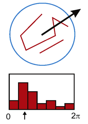
Orientation Assignment
- Scale-space extrema detection
- Keypoint localization
- Orientation assignment Compute best orientations(s) for each keypoint region.
- Keypoint description Use local image gradients at selected scale and rotation to describe each keypoint region
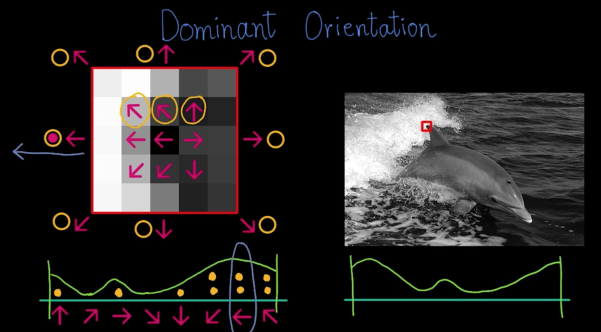
Descriptors Invariant to Rotation
- Find the dominant direction of gradient - that is the base orientation
- Compute image derivatives relative to this orientation

**Quiz**
What is the dominant oritentation for the image below?
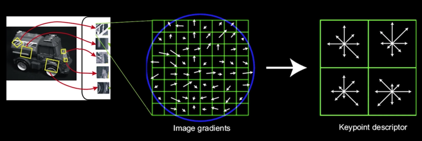
4. Keypoint Descriptors
- Next is compute a descriptor for the local image region about each keypoint that is:
- Highly distinctive
- As invariant as possible to variations such as changes in viewpoint and illumination
But first... normalization...
- Rotate the window to standard orientation
- Scale the window size based on the scale at which the point was found
Compute a feature vector based upon:
- Histogram of gradients
- weighted by the magnitude of the gradient
Smoothness
The smoothness allows you to get slow change in the descriptor as you move just a little bit

Reduce effect of illumination
- Clip gradient magnitudes to avoid excessive influence of high gradients
- after rotation normalization, clamp gradients > 0.2
- 128-dim vector normalized to magnitude 1.0
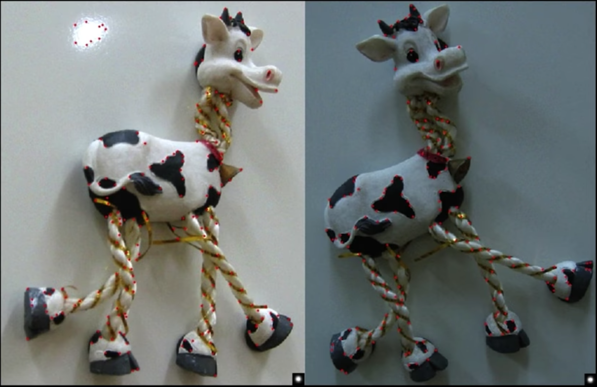
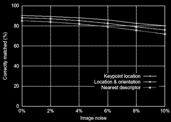
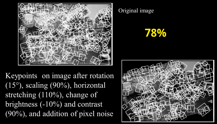
Evaluating the SIFT descriptors
- Database images were subjected to rotation, scaling, affine, stretch, brightness, and contrast changes, and added noise
- Feature point detectors and descriptors were compared before and after the distortions
- Mostly looking for stability with respect to change

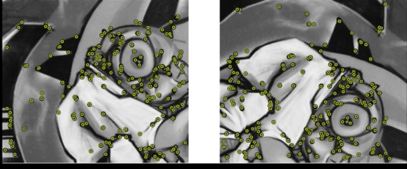
Experimental Results


In [156]:
## We will test SIFT on the following images that were drawn randomly from the internet
imgs = [imread("imgs/ev_sift%d.jpg" % i) for i in range(1,5)]
fig = plt.gcf()
fig.set_size_inches((20,15))
plt.subplot(221).imshow(imgs[0])
plt.subplot(222).imshow(imgs[1])
plt.subplot(223).imshow(imgs[2])
plt.subplot(224).imshow(imgs[3])
Out[156]:

In [28]:
def gen_sift_features(gray_img):
sift = cv.xfeatures2d.SIFT_create()
kp, desc = sift.detectAndCompute(gray_img, None)
return kp, desc
def show_sift_features(gray_img, color_img, kp,ax):
fig = plt.gcf()
fig.set_size_inches((20,8))
return ax.imshow(cv.drawKeypoints(gray_img, kp, color_img.copy()))
In [158]:
sifts = [gen_sift_features(gray(img)) for i in imgs]
In [159]:
fig = plt.gcf()
fig.set_size_inches((20,40))
show_sift_features(gray(imgs[0]), imgs[0], sifts[0][0],ax=plt.subplot(411))
show_sift_features(gray(imgs[1]), imgs[1], sifts[1][0],ax=plt.subplot(412))
show_sift_features(gray(imgs[2]), imgs[2], sifts[2][0],ax=plt.subplot(413))
show_sift_features(gray(imgs[3]), imgs[3], sifts[3][0],ax=plt.subplot(414))
Out[159]:

**Not Quite Impressive**
Feature Matching Using SIFT
In [130]:
messi = imgs[1]
imshow(messi)

In [140]:
messi_name = messi[80:105,140:200]
imshow(messi_name)

In [147]:
kp1,desc1 = gen_sift_features(gray(messi_name))
In [148]:
show_sift_features(gray(messi_name), messi_name, kp,ax=plt.subplot())
Out[148]:

Nearest Neighbor
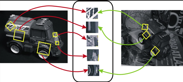
- Better: hypotheses are generated by approximate nearest neighbor matching of each feature to vectors in the database
- SIFT uses best-bin-first (Beis & Lowe, 97) modification to k-d tree algorithm
- Use heap data structure to identify bins in order by their distance from query point
Nearest-neighbor matching to feature database
- Result: can give speedup by factor of 100-1000 while finding nearest neighbor (of interest) 95% of the time
Nearest-neighbor technique

Wavelet-Based Hashing
Compute a short (3-vector) descriptor from the neightborhood using a Haar "wavelet"
Quantize each value into 10 (overlapping) bins ($10^3$ total entries)

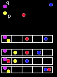
Locality Sensitive Hashing
Idea: construct hash function g: $\color{blue}{R^d \rightarrow U}$ such that for any points p,q:
- If $\color{blue}{D(p,q) \leq r}$, then Pr[g(p)=g(q)] is
"high""not-so-small" - If $\color{blue}{D(p,q) > cr}$, then Pr[g(p)=g(q)] is "small"
- If $\color{blue}{D(p,q) \leq r}$, then Pr[g(p)=g(q)] is
Then we can solve the problem by hashing
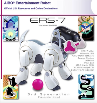
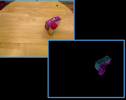
3D Object Recognition


Code Time
In [29]:
messi = imread("imgs/ev_sift2.jpg")
messi_kp, messi_desc = gen_sift_features(gray(messi))
imshow(messi)
show_sift_features(gray(messi), messi, messi_kp,ax=plt.subplot())
Out[29]:

In [30]:
messi_name = messi[80:105,140:200]
imshow(messi_name)
In [31]:
messiname_kp,messiname_desc = gen_sift_features(gray(messi_name))
show_sift_features(gray(messi_name), messi_name, messname_kp,ax=plt.subplot())
Out[31]:

Using KNN
In [32]:
# BFMatcher with default params
bf = cv.BFMatcher()
matches = bf.knnMatch(messiname_desc,messi_desc, k=2)
# Apply ratio test
good = []
for m,n in matches:
if m.distance < 0.75*n.distance:
good.append([m])
# cv.drawMatchesKnn expects list of lists as matches.
img3 = cv.drawMatchesKnn(messi_name,messiname_kp,messi,messi_kp,good,None,flags=2)
fig = plt.gcf()
fig.set_size_inches((20,8))
plt.imshow(img3),plt.show()

Out[32]:
Using FLANN
In [33]:
FLANN_INDEX_KDTREE = 0
index_params = dict(algorithm = FLANN_INDEX_KDTREE, trees = 5)
search_params = dict(checks=50) # or pass empty dictionary
flann = cv2.FlannBasedMatcher(index_params,search_params)
matches = flann.knnMatch(messiname_desc,messi_desc,k=2)
# Need to draw only good matches, so create a mask
matchesMask = [[0,0] for i in range(len(matches))]
# ratio test as per Lowe's paper
for i,(m,n) in enumerate(matches):
if m.distance < 0.7*n.distance:
matchesMask[i]=[1,0]
draw_params = dict(matchColor = (0,255,0),
singlePointColor = (255,0,0),
matchesMask = matchesMask,
flags = 0)
img3 = cv2.drawMatchesKnn(messi_name,messiname_kp,messi,messi_kp,matches,None,**draw_params)
fig = plt.gcf()
fig.set_size_inches((20,40))
plt.imshow(img3,),plt.show()

Out[33]:
Lets rotate the image, and scale it and see if it is able to find Messi's name
In [140]:
import scipy.ndimage
rmessi = scipy.ndimage.rotate(messi,-50,cval=255)
imshow(rmessi)

In [141]:
rmessi_kp, rmessi_desc = gen_sift_features(gray(rmessi))
imshow(rmessi)
show_sift_features(gray(rmessi), rmessi, rmessi_kp,ax=plt.subplot())
Out[141]:

In [142]:
# BFMatcher with default params
bf = cv.BFMatcher()
matches = bf.knnMatch(messiname_desc,rmessi_desc, k=2)
# Apply ratio test
good = []
for m,n in matches:
if m.distance < 0.75*n.distance:
good.append([m])
# cv.drawMatchesKnn expects list of lists as matches.
img3 = cv.drawMatchesKnn(messi_name,messiname_kp,rmessi,rmessi_kp,good,None,flags=2)
fig = plt.gcf()
fig.set_size_inches((20,8))
plt.imshow(img3),plt.show()

Out[142]:
Great. Lets scale it
In [143]:
smessi = rmessi[::2,::2] ## scaling by 1/2
smessi_kp, smessi_desc = gen_sift_features(gray(smessi))
imshow(smessi)
# BFMatcher with default params
bf = cv.BFMatcher()
matches = bf.knnMatch(messiname_desc,smessi_desc, k=2)
# Apply ratio test
good = []
for m,n in matches:
if m.distance < 0.75*n.distance:
good.append([m])
# cv.drawMatchesKnn expects list of lists as matches.
img3 = cv.drawMatchesKnn(messi_name,messiname_kp,smessi,smessi_kp,good,None,flags=2)
fig = plt.gcf()
fig.set_size_inches((20,8))
plt.imshow(img3),plt.show()


Out[143]:
Was not found. Lets see why
In [144]:
## Stolen from L2.ipynb
def display_pair(imgs,titles):
plt.gray()
plt.figure(figsize=(20,20))
plt.subplot(121)
ax = plt.gca()
ax.xaxis.set_major_locator(plt.NullLocator())
ax.yaxis.set_major_locator(plt.NullLocator())
plt.imshow(imgs[0])
plt.title(titles[0], size=20)
if len(imgs)> 1:
plt.subplot(122)
plt.imshow(imgs[1])
plt.title(titles[1], size=20)
ax = plt.gca()
ax.xaxis.set_major_locator(plt.NullLocator())
ax.yaxis.set_major_locator(plt.NullLocator())
plt.show()
rotated = cv.drawKeypoints(gray(rmessi), rmessi_kp, rmessi.copy())
scaled = cv.drawKeypoints(gray(smessi), smessi_kp, smessi.copy())
rotated_name = rotated [150:220,330:400]
scaled_name = scaled[70:110,150:190]
display_pair([rotated_name,scaled_name],["Rotated","Scaled"])

As it appears from above, the reason is that, unlike the rotate version, when we scaled down the image, only two feature points were detected around Messi's name and thus the template couldn't be matched.
🤩🎩👏🏻 Last day of 2018. Messi finished the year of 2018 as the top scorer. He scored 51 goals. Moreover, while he had tough year in terms of teams' trophies, he was, as always at his top level, and continued to entertain, equally, his lovers and his haters. 🤩🎩👏🏻
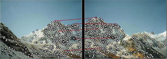
Feature Based Alignment
Review: Overall Strategy
- Compute features - detect and describe
- Find some useful matches: kd-tree, best-bin, hashing
- Compute and apply the best transformation: e.g. affine, translation, or homography
Featured-based alignment algorithm
Extract Features

Fig.30(a) Compute putative matches - e.g. "closest descriptor" kd-tree, best bin, etc...
- Loop until happy:
- Hypothesize transformation T from some matches
- Verify transformation (search for other matches consistent with T) - mark best

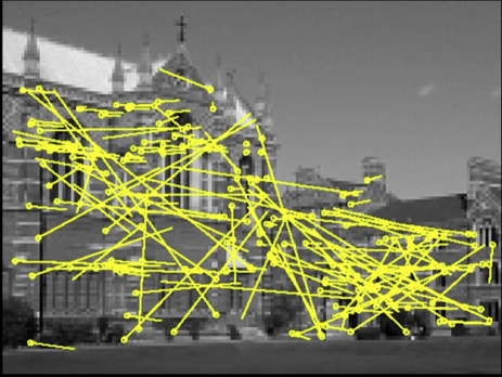
Feature Matching
- Exhaustive search
- Hashing
- Nearest neighbor techniques
.... but these give the best match. How do we know it's a good one?
Feature-space outlier rejection
- Let's not match all features, but only these that have "similar enough" matches
- How can we do it?
- SSD(patch1,patch2)<threshold
- How to set threshold

Feature Matching Problem
- Exhaustive search
- Hashing
- Nearest neighbor techniques
But...remember the distinctive vs invatiant competition? implies:
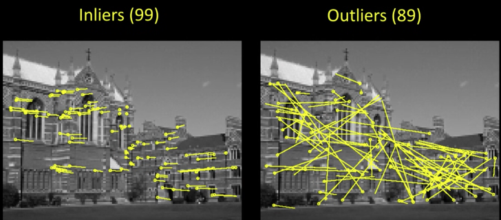
Problem: Even when pick best match, still lots (and lots) of wrong matches - "outliers". What should we do?
Typical least squares line fitting
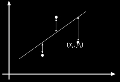
$$\color{blue}{E = \sum^{n}_{i=1} \left(y_i - \begin{bmatrix}x_i &1\end{bmatrix}\begin{bmatrix}m\\ b\end{bmatrix}\right)^2 = \left\vert\left\vert\begin{bmatrix}y_1\\.\\.\\.\\y_n\end{bmatrix}-\begin{bmatrix}x_1&1\\.&.\\.&.\\.&.\\x_n&1\end{bmatrix}\begin{bmatrix}m\\ b\end{bmatrix}\right\vert\right\vert^{2} = ||y - Xh||^2 }$$
$$\color{blue}{E = (y-Xh)^T(y-Xh) = y^Ty - 2(Xh)^Ty + (Xh)T(Xh)}$$
$$\color{blue}{\implies \frac{dE}{dh} = 2X^TXh - 2X^Ty = 0}$$ $$\color{blue}{\implies X^TXh = X^Ty}$$ $$\color{blue}{\implies h = (X^TX)^-1X^Ty}$$
In [157]:
import statsmodels.api as sm
import numpy as np
import matplotlib.pyplot as plt
X = np.random.rand(100)
Y = X + np.random.rand(100)*0.1
# Ordinary least squares
results = sm.OLS(Y,sm.add_constant(X)).fit()
print (results.params)
plt.scatter(X,Y)
X_plot = np.linspace(0,1,100)
plt.plot(X_plot, X_plot*results.params[1] + results.params[0])
plt.show()

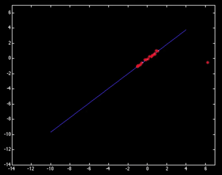
In [209]:
import matplotlib.pyplot as plt
X = np.random.rand(100)
Y = X + np.random.rand(100)*0.1
X_plot = np.linspace(0,1,100)
fig,ax = plt.subplots(ncols=2,nrows=2)
fig.set_size_inches((20,10))
# Ordinary least squares
results = sm.OLS(Y,sm.add_constant(X)).fit()
ax[0,0].scatter(X,Y)
ax[0,0].plot(X_plot, X_plot*results.params[1] + results.params[0])
Y[np.argmax(X)] = 100
results = sm.OLS(Y,sm.add_constant(X)).fit()
ax[0,1].scatter(X,Y)
ax[0,1].plot(X_plot, X_plot*results.params[1] + results.params[0])
X = np.random.normal(1,0.0001,100)
Y = np.random.rand(100)
results = sm.OLS(Y,sm.add_constant(X)).fit()
print(results.params)
ax[1,0].set_title("Vertical points")
ax[1,0].scatter(X,Y)
ax[1,1].set_title("Bad fitting for the points on the left")
ax[1,1].plot(X, X*results.params[1] + results.params[0])
plt.show()

Total least squares
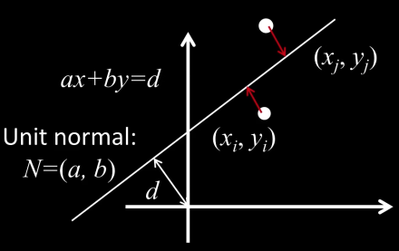
$$\color{blue}{\frac{\partial E}{\partial d} = \sum_{i=1}^n{}-2(ax_i + by_i -d )=0}$$ $$\color{blue}{\implies d = \frac{a}{n}\sum_{i=1}^{n}x_i +\frac{b}{n}\sum_{i=1}^{n}x_i = a\bar{x}+b\bar{y}}$$ $$\color{blue}{E = \sum_{i=1}^{n}(a(x_i-\bar{x}) + b(y_i-\bar{y}))^2 = \left\vert\left\vert\begin{bmatrix}x_1-\bar{x}&y_1-\bar{y}\\.&.\\.&.\\.&.\\x_n-\bar{x}&y_n-\bar{y}\end{bmatrix}\begin{bmatrix}a\\b\end{bmatrix}\right\vert\right\vert^2 = (Uh)^T(Uh)}$$
$$\color{blue}{\implies \frac{dE}{dh} = 2(U^TU)h = 0}$$
Solution to $(U^TU)h = 0$, subject to $||h||^2 = 1$:
eigenvector of $U^TU$ associated with the smalles eigenvalue (Again SVD to least squares solution to homogeneous linear system)


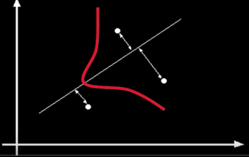
Robust Estimators
- General approach: minimize $\color{blue}{\sum_{i}\rho(r_i(x_i,\theta);\sigma)}$
- $\color{blue}{r_i(x_i,\theta)}$ - residual of $\color{blue}{i^{th}}$ point w.r.t. model parameters $\color{blue}{\theta}$
- $\color{blue}{\rho}$ - robust function with scale parameter $\color{blue}{\sigma}$

The Robust function $\rho$ behaves like squared distance for small values of the residual $u$ but saturates for larger values of $u$
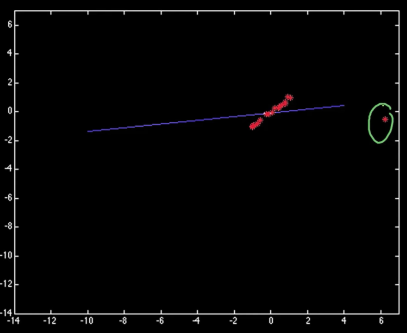
Choosing the scale: Just right
Choosing the scale: Too small
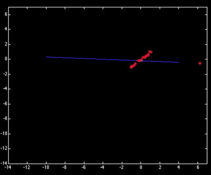
In [440]:
X = np.random.normal(0,2,100)
Y = X + np.random.normal(0,0.5,100)
X_plot = np.linspace(-5,20,100)
fig,ax = plt.subplots(ncols=2,nrows=2)
fig.set_size_inches((20,10))
results = sm.OLS(Y,sm.add_constant(X)).fit()
ax[0,0].scatter(X,Y)
ax[0,0].plot(X_plot, X_plot*results.params[1] + results.params[0])
X[-1] = 50
Y[np.argmax(X)] = 2
results = sm.OLS(Y,sm.add_constant(X)).fit()
ax[0,1].scatter(X,Y)
ax[0,1].plot(X_plot, X_plot*results.params[1] + results.params[0])
def gen_data(t, a, b, c, noise=0, n_outliers=0, random_state=0):
y = a + b * np.exp(t * c)
rnd = np.random.RandomState(random_state)
error = noise * rnd.randn(t.size)
outliers = rnd.randint(0, t.size, n_outliers)
error[outliers] *= 10
return y + error
from scipy.optimize import least_squares
def fun(x, t, y):
return x[0] + x[1] * np.exp(x[2] * t) - y
x0 = np.array([1, 1, 1])*0.20
res_lsq1 = least_squares(fun, x0, args=(X, Y))
y_lsq = gen_data(X_plot, *res_lsq1.x)
ax[1,0].scatter(X,Y)
ax[1,0].plot(X_plot, y_lsq)
x0 = np.array([1, 1, 1])*2
res_lsq2 = least_squares(fun, x0, args=(X, Y))
y_lsq = gen_data(X_plot, *res_lsq2.x)
ax[1,1].scatter(X,Y)
ax[1,1].plot(X_plot, y_lsq)
Out[440]:

Find Consistent Matches
- Some "best" matches are correct
- Some are not. And the "not" are not part of any other consistent match...
- Need to find the right ones so can compute the pose/transform/fundamental... the model
- Today: Random Sample Consensus (RANSAC)
RANSAC: main idea
- Fitting a line (model) is easy if we know which points belong and which do not.
- If we had a proposed line (model), we could probably guess which points belong to that line (model): inliers
- Random Sample Consensus: randomly pick some points to define your line (model). Repeat enough times until you find a good line (model) - on with many inliers.
- Fishler & Bolles 1981 - Copes with a large proportion of outliers
RANSAC for general model
A given model type has a minimal set- the smallest number of samples from which the model can be computed.
- Line: 2 points
Image transformation are models. Minimal set of s of point pairs/matches:
- Translation: pick one pair of matched points
- Homography (for plane) - pick 4 point pairs
- Fundamental matrix - pick 8 point pairs (really 7 but lets not go there)
General RANSAC algorithm
- Randomly select s of point (or point pairs) to form a sample
- Instantiate the model
- Get consensus set $C_i$- the points whithin error bounds (distance threshold) of the model
Choosing the parameters
- Initial number of points in the minimal set $s$
- Typically minimum number needed to fit the model
- Distance threshold $t$
Distance Threshold
- Let's assume location noise is Gaussian with $\color{blue}{\sigma^2}$
- Then the distance $d$ has Chi distribution with k degrees of freedoms where $k$ is the dimension of the Gaussian.
- If one dimension, e.g. distance off a line, then 1DOF
$$\color{blue}{f(d) = \frac{\sqrt{2}e^{-(\frac{d^2}{2\sigma^2})}}{\sqrt{\pi}\sigma},d\ge 0}$$
For 95% comulative threshold $\color{blue}{t}$ when Gaussian with $\sigma$:$t^2$ = 3.84$\color{blue}{\sigma^2}$
That is: if $t^2$- 3.84$\color{blue}{\sigma^2}$ then 95% probability that $d
Choosing the parameters
- Initial number of points in the minimal set $s$
- Typically minimum number needed to fit the model
- Distance threshold $\color{blue}{t}$
- Choose $t$ so probability for inlier is hight (e.g. 0.95)
- Zero-mean Gaussian noise with std. dev. $\sigma$: $\color{blue}{t^2}$ = $\color{blue}{3.84\sigma^2}$
- Number of Samples N
- Choose $N$ so that, with probability $\color{blue}{p}$, at least one random sample set is free from outliers (e.g. $\color{blue}{p = 99}$)
- Need to set $\color{blue}{N}$ based upon the outlier ration $\color{blue}{e}$
Calculate N
- $\color{blue}{s}$- number of points to compute solution
- $\color{blue}{p}$- probability of success
- $\color{blue}{e}$- proportion outliers, so % $\color{blue}{inliers = (1-e)}$
- P (sample set with all inliers) = $\color{blue}{(1-e)^s}$
- P (sample set will have at least one outlier) = $\color{blue}{(1-(1-e)^s)}$
- P (all N samples have outlier) = $\color{blue}{(1-(1-e)^s)^N}$
- We want P (all N samples have outlier) < $\color{blue}{(1-p)}$
- So $\color{blue}{(1- (1 - e)^s)^N < (1-p)}$
$$\color{blue}{N > log(1-p)/log(1-(1-e)^s)}$$
What does N Look Like
- set p = 0.99 - chance of getting good sample
$s=2, e= 5\% \implies N = 2$
$s=2, e= 50\% \implies N = 17$Line
$s=4, e= 5\% \implies N = 3$
$s=4, e= 50\% \implies N = 72$ Homography
$s=8, e= 5\% \implies N = 5$
$s=8, e= 50\% \implies N = 1177$Fundamental Matrix
- N increases steeply with s
In [496]:
import pandas as pd
f = lambda p,s,e: 1+int(np.log(1-p)/np.log(1-np.power((1-e),s)))
s = [2,3,4,5,6,7,8]
e = [0.05,0.1,0.2,0.25,0.30,0.40,0.5]
p = 0.99
table = [[f(p,si,ei) for ei in e] for si in s]
table
Out[496]:
In [472]:
x = np.arange(0.1,0.8,0.01)
y = [f(0.99,4,xi) for xi in x]
plt.plot(x,y)
Out[472]:

How big does N need to be?
$$\color{blue}{N > log(1-p)/log(1-(1-e)^s)}$$
$\color{blue}{N = f(e,s,p)}$, but not the number of points!
In [529]:
import random
imgLeft = imread("imgs/matching_feature_ransac1.png")
imgRight = imread("imgs/matching_feature_ransac2.png")
fig,ax = plt.subplots(ncols=2)
fig.set_size_inches((20,15))
cPointsLeft = [(200,75),(165,115),(200,140),(167,165),(182,190)]
cPointsRight = [(85,78),(52,117),(89,141),(50,162),(67,188)]
bPointsLeft = [(115,75),(115,135)]
bPointsRight = [(137,75),(90,140)]
colors = [(random.randint(0,256),random.randint(0,256),random.randint(0,256))
for i in range(len(pointsLeft+bPointsLeft))]
for i,p in enumerate(cPointsLeft+bPointsLeft):
imgLeft = cv2.circle(imgLeft,(p[0],p[1]),5,colors[i],-11)
for i,p in enumerate(cPointsRight+bPointsRight):
imgRight = cv2.circle(imgRight,(p[0],p[1]),5,colors[i],-11)
ax[0].imshow(imgLeft)
ax[1].imshow(imgRight)
Out[529]:

RAndom SAmple Consensus (1)
Select one match, count inliers
In [530]:
def dfScatter(df, xcol='TX', ycol='TY', catcol='correct'):
fig, ax = plt.subplots()
categories = np.unique(df[catcol])
colors = np.linspace(0, 1, len(categories))
colordict = dict(zip(categories, colors))
df["Color"] = df[catcol].apply(lambda x: colordict[x])
ax.scatter(df[xcol], df[ycol], c=df.Color)
return fig
In [531]:
d = []
for pl,pr in zip(cPointsLeft,cPointsRight):
d.append({"x1":pl[0],"y1":pl[1],"x2":pr[0],"y2":pr[1],"correct": True })
for pl,pr in zip(bPointsLeft,bPointsRight):
d.append({"x1":pl[0],"y1":pl[1],"x2":pr[0],"y2":pr[1],"correct": False })
df = pd.DataFrame(d)
In [532]:
print(df)
df["TX"] = np.abs(df["x2"]-df["x1"])
df["TY"] = np.abs(df["y2"]-df["y1"])
df["Color"] = df["correct"].apply(lambda x: "blue" if x else "red")
df.plot.scatter(x="TX",y="TY",c=df.Color)
Out[532]:

In [543]:
def count_inliers(df,selected,threshold,imgL,imgR):
s = df.iloc[selected]
df["Inlier"] = df.apply(lambda x: (x["TX"]-s["TX"])**2 + (x["TY"]-s["TY"])**2 < threshold,axis=1)
fig,ax = plt.subplots(ncols=2)
fig.set_size_inches((20,15))
colors = df.apply(lambda x: (0,0,255) if x["Inlier"] else (255,0,0),axis=1)
imgLeft = imgL.copy()
imgRight = imgR.copy()
for i in range(df.shape[0]):
r = df.iloc[i]
imgLeft = cv2.circle(imgLeft,(r["x1"],r["y1"]),5,colors[i],-11)
imgRight = cv2.circle(imgRight,(r["x2"],r["y2"]),5,colors[i],-11)
ax[0].imshow(imgLeft)
ax[1].imshow(imgRight)
In [552]:
imgLeft = imread("imgs/matching_feature_ransac1.png")
imgRight = imread("imgs/matching_feature_ransac2.png")
count_inliers(df,1,50,imgLeft,imgRight)

RAndom SAmple Consensus (2)
In [551]:
imgLeft = imread("imgs/matching_feature_ransac1.png")
imgRight = imread("imgs/matching_feature_ransac2.png")
count_inliers(df,6,50,imgLeft,imgRight)

Least squares fit
Find "average" translation vector
In [553]:
imgLeft = imread("imgs/matching_feature_ransac1.png")
imgRight = imread("imgs/matching_feature_ransac2.png")
count_inliers(df,1,50,imgLeft,imgRight)
In [558]:
inliers = df[df["Inlier"]]
avrgx, avrgy = inliers["TX"].sum()/inliers.shape[0],inliers["TY"].sum()/inliers.shape[0]
print ("The translation vector is (",avrgx, avrgy,")")
RANSAC for extimating homography
RANSAC loop:
- Select for feature pairs (at random)
- Compute homography H (exact)
- Compute inliers where SSD $(p'_i,Hpi)<\epsilon$
- Keep largest set of inliers
- Re-compute least-squares H estimate on all of the inliers
In [563]:
def detectAndDescribe(image):
# convert the image to grayscale
gray = cv2.cvtColor(image, cv2.COLOR_BGR2GRAY)
# detect and extract features from the image
descriptor = cv2.xfeatures2d.SIFT_create()
(kps, features) = descriptor.detectAndCompute(image, None)
# convert the keypoints from KeyPoint objects to NumPy
# arrays
kps = np.float32([kp.pt for kp in kps])
# return a tuple of keypoints and features
return (kps, features)
def matchKeypoints(kpsA, kpsB, featuresA, featuresB,
ratio, reprojThresh):
# compute the raw matches and initialize the list of actual
# matches
matcher = cv2.DescriptorMatcher_create("BruteForce")
rawMatches = matcher.knnMatch(featuresA, featuresB, 2)
matches = []
# loop over the raw matches
for m in rawMatches:
# ensure the distance is within a certain ratio of each
# other (i.e. Lowe's ratio test)
if len(m) == 2 and m[0].distance < m[1].distance * ratio:
matches.append((m[0].trainIdx, m[0].queryIdx))
# computing a homography requires at least 4 matches
if len(matches) > 4:
# construct the two sets of points
ptsA = np.float32([kpsA[i] for (_, i) in matches])
ptsB = np.float32([kpsB[i] for (i, _) in matches])
# compute the homography between the two sets of points
(H, status) = cv2.findHomography(ptsA, ptsB, cv2.RANSAC,
reprojThresh)
# return the matches along with the homograpy matrix
# and status of each matched point
return (matches, H, status)
# otherwise, no homograpy could be computed
return None
def drawMatches(imageA, imageB, kpsA, kpsB, matches, status):
# initialize the output visualization image
(hA, wA) = imageA.shape[:2]
(hB, wB) = imageB.shape[:2]
vis = np.zeros((max(hA, hB), wA + wB, 3), dtype="uint8")
vis[0:hA, 0:wA] = imageA
vis[0:hB, wA:] = imageB
# loop over the matches
for ((trainIdx, queryIdx), s) in zip(matches, status):
# only process the match if the keypoint was successfully
# matched
if s == 1:
# draw the match
ptA = (int(kpsA[queryIdx][0]), int(kpsA[queryIdx][1]))
ptB = (int(kpsB[trainIdx][0]) + wA, int(kpsB[trainIdx][1]))
cv2.line(vis, ptA, ptB, (0, 255, 0), 1)
# return the visualization
return vis
In [568]:
imgLeft = imread("imgs/matching_feature_ransac1.png")
imgRight = imread("imgs/matching_feature_ransac2.png")
kpl,descl = detectAndDescribe(imgLeft)
kpr,descr = detectAndDescribe(imgRight)
## H is the homography
m,H,status = matchKeypoints(kpl,kpr,descl,descr,ratio=0.75, reprojThresh=4.0)
imshow(drawMatches(imgLeft,imgRight,kpl,kpr,m,status))
H

Out[568]:
Adaptive Procedure
Adaptively determining the number of samples
- Inlier ratio $e$ is often unknown a priori
- Pick worst case, e.g. 50% ($e$ = 0.5) and adapt if more inliers are found
e.g. 80% inliers wourld yeald $e$ = 0.2
Adaptive procedure:
- $\color{blue}{N = \infty}$, $\color{blue}{\text{sample_count}=0}$, $\color{blue}{e = 1.0}$
- While $\color{blue}{N > \text{sample_count}}$
- Choose a sample and count the number of inliers
- Set $\color{blue}{e_0 = 1- \frac{number of inliers}{total number of points}}$
- If $\color{blue}{e_0<e}$ set $\color{blue}{e = e_0}$ and recompute $\color{blue}{N}$ from $\color{blue}{e}$: $$\color{blue}{N = \frac{log(1-p)}{log(1-(1-e)^s)}}$$
- Increment the sample_count by 1


In [569]:
## Any one is welcome to create the previous images in code
RANSAC Conclusion
The good
- Simple and general
- Applicable to many different problems, often works well in practice
- Robust to large numbers of outliers
- Applicable for larger number of parameters than Hough transform
- Parameters are easier to choose than Hough transform
The not-so-good
- Computational time grows quickly with the number of model parameters
- Not as good for getting multiple fits
- Really not good for approximate models
Common application
- Computing a homography (e.g., image stitching) or other image transform
- Estimating fundamental matrix( relating two views)
- Pretty much every problem in robot vision