=====================================

3A - L1 Camera and Images

=====================================

What is an image?

• In previous lesson: a function- a 2D pattern of intensity values
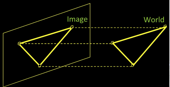
• Here: 1 2D projection of 3D points

First known Photograph - Heliograph

The first photograph was taken by Joseph Nicephore Niepce in 1826. The below image is a reproduction made in 1952

Fig.1 The reproduction of the first photograph Source

Imaging System

What is a camera?

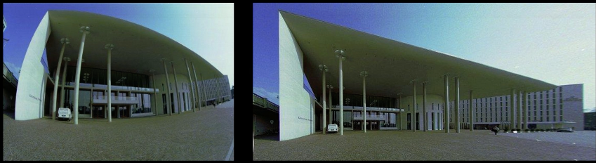
It's some device that allows the **projection** of light from three dimensions, to some medium (film, sensor,..etc) that will record the light pattern.

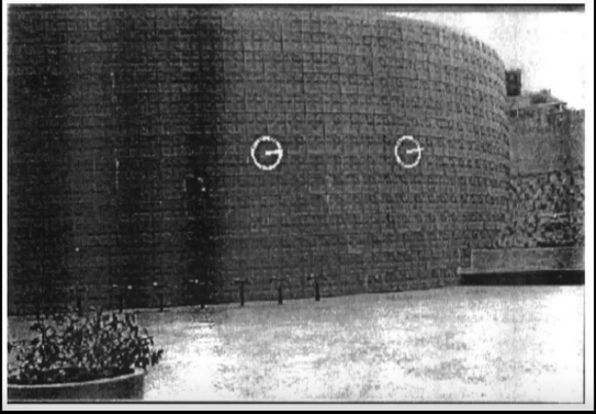
When you project a scene to the camera, you lose 3D information, and you have to find out what went out in the lost dimesnion. For instance, the image below were taken by a camera from front and right side. The projection from the right side shows the realistic depection of the globe painted on the side walk.

Fig.2(a) Example of projection. Notice the strange guy at the top of the globe

Fig.2(b) The real view of the projection as appears from right side

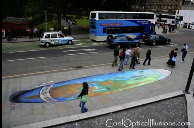
Image Formation

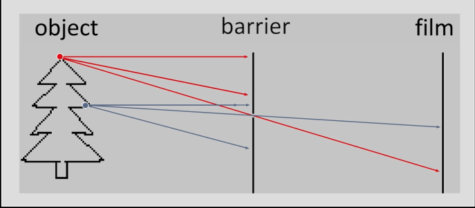
As shown in figure 3(a), a light is reflected from a point to a film will create an image. However, a single point will reflect lights all over the film. In order to solve this problem, we place a barrier, with a small holes (aperture) in it that each will allow single light through it to the film as in figure 3(b)

Fig.3(a) Light comes from a point poroject all over the film

Fig.3(b) A barrier with small holls (aperture) is placed between the scene and the film to allow only single light angle to the film

Aperture

How does aperture affect the image that we see? How does the size affect the image?

The bluriness of the image is directly related to the size of the arpeture. As the arpeture size decreases, the bluriness decrease and the crisper images are produced. Aperture sizes are in mm (e.g. 2mm, 1mm, 0.6mm, and 0.35mm)

Why not making the size very very small?

Because of diffraction effect due to the wave nature of light.

Fig.4 effect of aperture size on the image source

Lenses

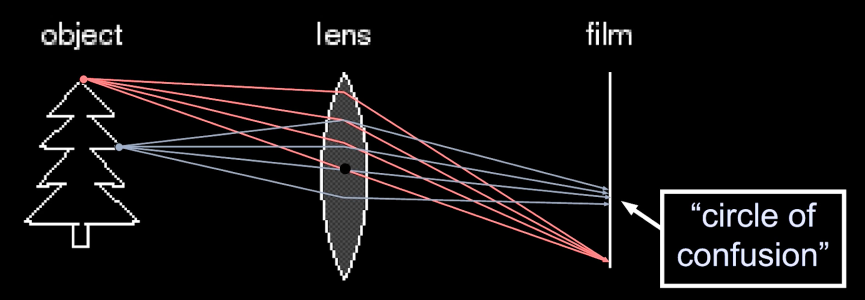
We don't really use pinhole cameras anymore. Instead, we use lenses. Lenses are desinged to project all lights comming from a point at a particular distance away to the same point on the film. However, as in Figure 5, the challange is that lights comming from different distance will be projected at slightly different points on the film (circle of confusion)

Fig.5(a): Shows lenses' concept and the circle of confusion

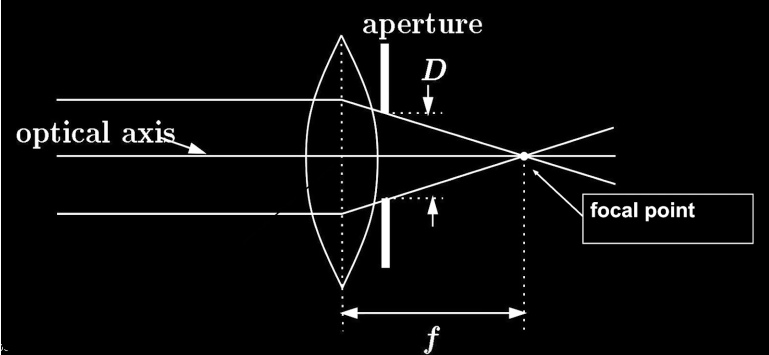
Lenses Components

• Optical axis: light passes straight through unbent
• Paralell lights are all bent to the same point
• Focal point: a point where parallel lights are bent to
• Aperture: to reduce the amount of spread of things, by restricting the set of rays that are coming in.

Fig.5(b): Shows lenses' components

Thin Lenses

Fig.6(a) depicts thin lenses

Fig.6(b) film lens diagram

Fig.6(c) film lens diagram

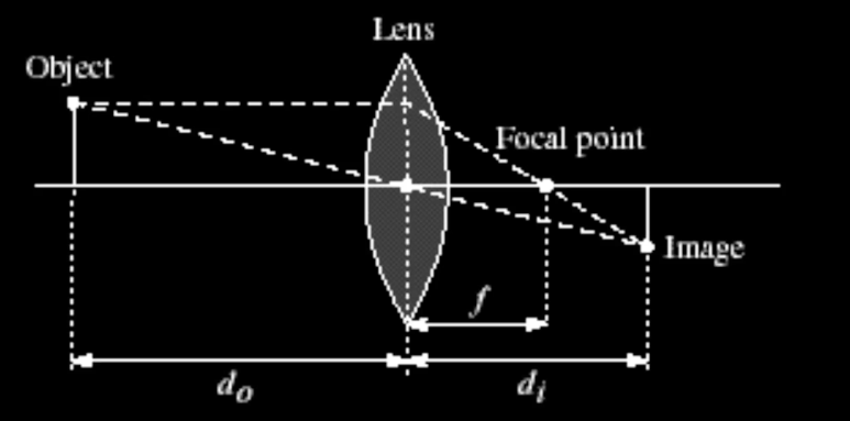
Can we predict the relationship between, say $\color{blue}{d_0}$ and $\color{blue}{d_i}$ given lens with a given focal point where $d_0$ is the distance of the object, and $d_i$ is the distance from the lens to the image (Figure 6(a))?

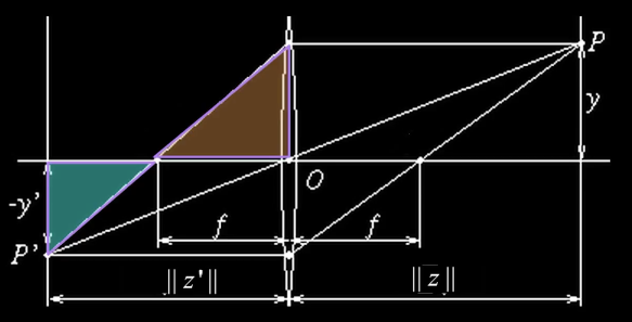
Using similar triangles in Figure 6(b), we can reason that given the point $P$ at $y$ and projected at point $P'$ at $-y$

$$\color{blue}{\frac{-y'}{y} = \frac{||z'||}{||z||}}$$

Also, using similar triangles in Figure 6(c), we can reason that

$$\color{blue}{\frac{-y'}{y} = \frac{||z'|| - f}{f}}$$

$$\color{blue}{\implies \frac{1}{||z||} = \frac{1}{f} - \frac{1}{||z'||}}$$

$$\color{blue}{\implies \frac{1}{f} = \frac{1}{||z||} + \frac{1}{||z'||}}$$

(Thin Lense Equation)

$y$: height of a point from the optical axis
$y'$: height of the projection of $P$ from the optical axis
$z$: distance to the world
$z'$: distance from lense to the image plane

So, any point that satisfy the thin lense Equation will be in focus. Hence, by moving the lense back and forward, we change where in the world things are in focus

Check out: http://www.phy.ntnu.edu.tw/ntnujava/index.php?topic=48

**Quize**

Fig.6(d): Thin lense quiz

f = 50.0
z = [1000.0,2000.0] # in mm
for zi in z:
    zp = 1/(1/f - 1/zi)
    print("When Z1 == %f, Z' == %f" % (zi,zp))

When Z1 == 1000.000000, Z' == 52.631579
When Z1 == 2000.000000, Z' == 51.282051

Varying Focus

Fig.7: The effect of varying focus Source

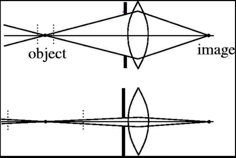
Depth of field

It is concerned with how much of focus change occurs for a certain point as the lense move in and out. The DoF is controlled by the aperture. With wide aperture, the rays diverge quite a bit, and hence moving the plane in a little bit cause the rays to spread out alot. On the other hand, with smaller aperture, the spread is much less as the plane is moving in (Figure 8a,b).

Fig.8 (a): depth of field Source

Fig.8 (b): change of aperture Source

Field of View (zooming)

How wide of a view do we have. There are two types of lens that can change their field of view:

1. changing focal lenght while staying in constant focus
2. changing focal length but must refocus (variable focal length lenses)

When the focal length is high, the angular deflection moves the pixels drastically and thus any shake in the camera will shake the image greatly. So the more the focal length, the more we need to stabilize the camera.

Fig.9 (a): change in field of view as we change focal length Source

Fig.9 (b): example change in field of view as we change focal length Source

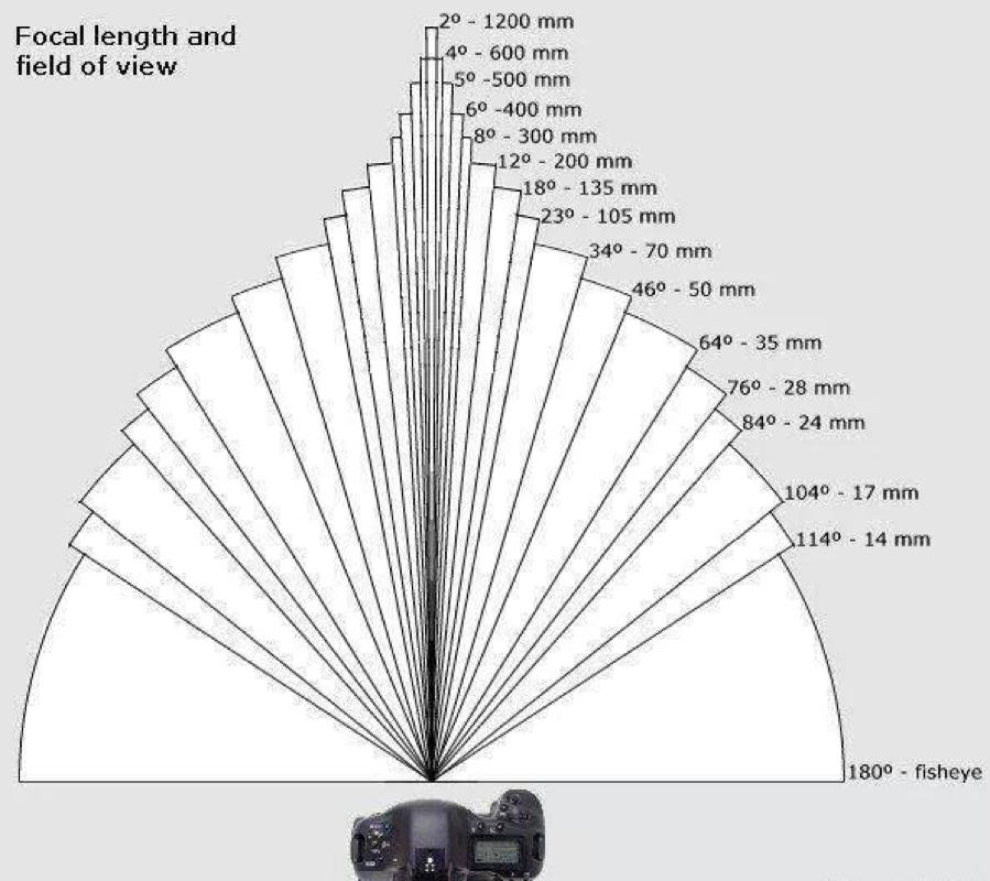
FOV depends on Focal Length

Fig.9 (c): Calculating FOV

The field of view can be calculated by calculating the angle $\color{blue}{\phi}$ depected in Figure 9(c).

$$\color{blue}{\phi = tan^-1(\frac{d/2}{f})}$$

$\color{blue}{d}$: the retina or sensor size

Larger Focul Length $\implies$ Smaller FOV
Bigger the imaging surface $\implies$ Bigger FOV

**Quize**

Fig.9(d): Field of view quiz

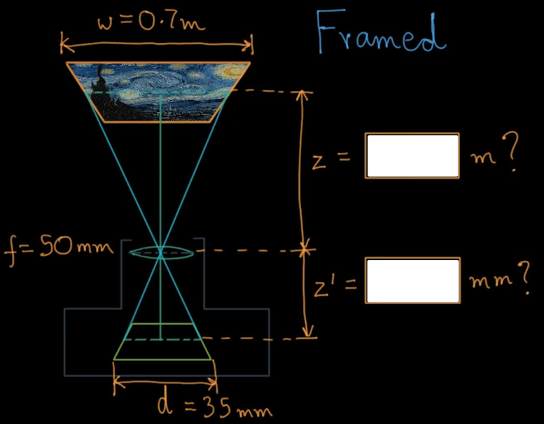
$$\color{blue}{\frac{1}{f} = \frac{1}{||z||} + \frac{1}{||z'||}}$$ $$\color{blue}{\implies \frac{1}{f} = \frac{z' + z}{z'z}}$$ $$\color{blue}{\implies fz' + fz = zz'}$$ $$\color{blue}{\implies fz' = zz' - fz}$$ $$\color{blue}{\implies fz' = z(z' - f)}$$ $$\color{blue}{\implies z = \frac{z'f}{z'-f} \,\,(1)}$$

$$\color{blue}{\frac{d/2}{z'} = \frac{w/2}{z}}$$ $$\color{blue}{\implies z = \frac{w/d}{z'} \,\,(2)}$$

from 1 & 2

$$\color{blue}{\implies \frac{z'f}{z'-f} = \frac{w/d}{z'}}$$ $$\color{blue}{\implies w(z'-f) = df}$$ $$\color{blue}{\implies z' -f = \frac{df}{w}}$$ $$\color{blue}{\implies z' = \frac{df}{w} + f}$$

import numpy as np
w = 0.7*1000 #to mm
f = 50
d = 35
zp = d*f/w + f ## df/w + f
z = zp*w/d ## z = z'w/d

print(z/1000,zp) # to m

1.05 52.5

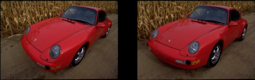
Zooming and Moving are not the same

In Figure 10(a), the image on the left image were taken with a large FOV, and small $f$ while the camera is close to the car. The image on the right, on the other hand, is taken with small FOV, and large $f$ while the camera is far from the car. You can notice that the shape is different. The left image has what is called Perspctive Distortion.

Figure 10(b) gives another example of Perspctive Distortion as we minimize $f$ and move closer to the face

Fig.10 (a): zooming vs moving

Fig.10 (b): zooming vs moving

Dolly Zoom

When the camera move closer and closer to an object while widening the lense at the same time, the object in the middle will have the same size, and to maintain its stationary point. However, this will create an illusionary scene where the stuff on the outside will grow.

Fig.11: Dolly Zoom

Lenses Are Not Perfect

There are many problems that might arise from lenses, photographers, or the scene.

Geometric Distortion

You can correct geometric distortion in post-imaging tools like photoshop if you know the focal length of your camera Figure 12(b)

Fig.12 (a): Geometric Distortion

Fig.12 (b): Correction of Radial Distortion

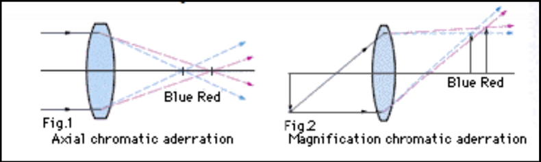
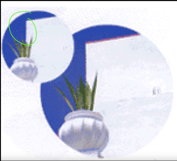
Chromatic Aberration

This problem happens when rays of different wavelength focus in different planes. The problem is how to get all lights from a certain point to land on same point on the image. Notice the red line in the bigger picture in Figure 12(d)

Fig.12 (c): Chromatic Aberration

Fig.12 (d): Chromatic Aberration Example

Vignetting

With some camera settings, not all rays that are hitting in the middle of the image are being caught at the corners.

Fig.12 (e): Vignetting Source

Fig.12 (f): Example of Vignetting Source

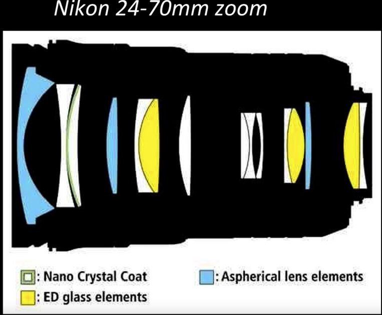
Lense Systems

Advanced cameras have multiple lenses. The camera in Figure 13 has 15 lenses that change according to the need.

Fig.13: Example of advanced camera lenses

=====================================

3A - L2 Perspective Imaging

=====================================

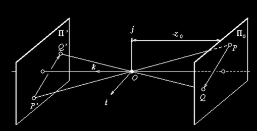
Coordinate Systems

• Using the pinhole model as an approximation
  • Put the optical center (Center of Projection) at the origin
  • Standard (x,y) Coordinate System
  • Put the image plane (Projection Plane) in front of the COP (for math convenient)
  • The cameral looks down the negative z axis

Fig.14: depects the coordinate system for modeling projection

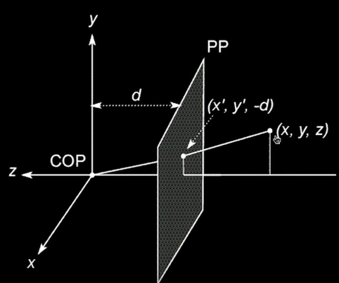
Projection Equations

• Compute intersection with Perspective Projection of ray from (x,y,z) to COP
• Derived using similar triangles

$$\color{blue}{(X,Y,Z) -> (-d\frac{X}{Z},-d\frac{Y}{Z},-d)}$$

So, we can get the projection by throwing out the last coordinate:

$$\color{blue}{(x', y') = (-d\frac{X}{Z},-d\frac{Y}{Z})}$$

**When dividing by Z, distant objects are smaller

**Quize**

When objects are very far away, the real X and real Z can be huge. If I move the camera (the origin), those numbers hardly change. This explains:

a) Why the moon follows you
b) Why the North Star is always North
c) Why you can tell time from the Sun regardless of where you are?
d) All of the above

Homogeneous Coordinates

Is this a linear transformation?
No- division by the (not constant) Z is non-linear

Trick: add one more coordinate:

Homogeneous image (2D) coordinates$\,\,\,(x,y)\,\,\, \Rightarrow \begin{bmatrix} x \\ y \\ 1\end{bmatrix} $

Homogeneous scene (3D) coordinates$\,\,\,(x,y,z) \Rightarrow \begin{bmatrix} x \\ y \\ z \\ 1\end{bmatrix} $

Converting from homogeneous coordinates:

$$\color{blue}{\begin{bmatrix} x \\ y \\ w\end{bmatrix} \,\,\, \Rightarrow \,\,\,(x/w,y/w)}$$

$$\color{blue}{\begin{bmatrix} x \\ y \\ z \\ w\end{bmatrix} \,\,\, \Rightarrow \,\,\,(x/w,y/w,z/w)}$$

**This makes homogenous coordinates invariant under scale

Perspective Projection

projetion is a matrix multiply using homogeneous coordinates:

$$\color{blue}{\begin{bmatrix} 1 & 0 & 0 & 0 \\ 0 & 1 & 0 & 0 \\ 0 & 0 & \frac{1}{f} & 0 \end{bmatrix}\begin{bmatrix} x \\ y \\ z \\ 1\end{bmatrix} = \begin{bmatrix} x \\ y \\ \frac{z}{f}\end{bmatrix} \,\,\, \Rightarrow \,\,\,(f\frac{x}{z},f\frac{y}{z})}$$

$$\color{blue}{\Rightarrow (u,v)}$$

$f$: is the focal length, the distance from the center of projection to the image plane

How does scaling the projection matrix change the transformation?

$$\color{blue}{\begin{bmatrix} f & 0 & 0 & 0 \\ 0 & f & 0 & 0 \\ 0 & 0 & 1 & 0 \end{bmatrix}\begin{bmatrix} x \\ y \\ z \\ 1\end{bmatrix} = \begin{bmatrix} fx \\ fy \\ z \end{bmatrix} \,\,\, \Rightarrow \,\,\,(f\frac{x}{z},f\frac{y}{f})}$$

**So invariant under scale

**Quize**

Given Point p in 3-space[x y z] and focal length f, write a function that returns the location of the projected point on 2D image plane [u v]

import numpy as np
def project(p,f):
    A = np.array([[1,0,0,0],[0,1,0,0],[0,0,1/f,0]])
    p = np.append(p,1)
    mul = np.matmul(A,p.T)
    return (mul[0]/mul[2],mul[1]/mul[2])

p1 = np.array([200,100,50])
p2 = np.array([200,100,100])
f = 50
print(project(p1,f))
print(project(p2,f))

(200.0, 100.0)
(100.0, 50.0)

Geometric properties of projection

• Points go to points
• Lines go to lines
• Polygons go to polygons

Fig.15: properties of projection

Parallel Lines in the World Meet in the Image (Vanishing) point

Line in 3-space

$$\color{blue}{x(t) = x_0 + at}$$ $$\color{blue}{y(t) = y_0 + bt}$$ $$\color{blue}{z(t) = z_0 + ct}$$

$\color{blue}{x_0, y_0,z_0}$: is starting point
$\color{blue}{at,bt,zt}$: moving on vector

Perspective projection of the line

$$\color{blue}{x'(t) = \frac{fx}{z} = \frac{f(x_{0} + at)}{z_0 + ct}}$$
$$\color{blue}{y'(t) = \frac{fy}{z} = \frac{f(y_{0} + bt)}{z_0 + ct}}$$

In the limit as $\color{blue}{t \rightarrow \pm}$ we have (for $\color{blue}{c \neq 0}$) :

$$\color{blue}{x'(t) \rightarrow \frac{fa}{c}, \,\,\,\, y'(t) \rightarrow \frac{fb}{c}}$$

regardless of their starting point (that is $\color{blue}{x_0\,\, and\,\, y_0}$)

Fig.16(a): Vanishing Point

Fig.16(b): Example of Vanishing Point

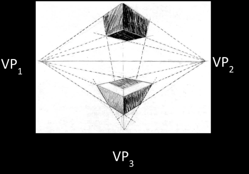
Vanishing Points

• Each set of parallel lines (=direction) meets at a different point.
  • The line is called the horizon for that plane

Fig.17 (a): set of parallel lines

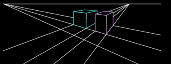
3-point perspective

Different directions correspond to different vanishing points

Fig.17(b): 3-point perspective

Fig.17(c): example of vanishing point

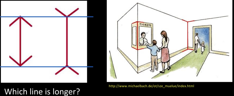
Human Vision (Muller-Lyer illusion)

Fig.18(a): illusion to human vision

Fig.18(b): illusion to human vision

**Quize**

What determines at what point in the image parallel lines intersect?

a) The direction the lines have in the world
b) Whether the world lines are on the ground plane
c) The orientation of the camera
d) (a) and (c)

Other models

Orthograpphic Projection

Special case of perspective projection

• Distance from the COP to the image plane is infinite
• Also called 'parallel projection': (x,y,z) -> (x,y)
• The projection matrix is:

$$\color{blue}{\begin{bmatrix} 1 & 0 & 0 & 0 \\ 0 & 1 & 0 & 0 \\ 0 & 0 & 0 & 1 \end{bmatrix}\begin{bmatrix} x \\ y \\ z \\ 1\end{bmatrix} = \begin{bmatrix} x \\ y \\ 1 \end{bmatrix} \,\,\, \Rightarrow \,\,\,(x,y)}$$

Fig.19(a): Orthograpphic Projection

Week Perspective

• Perspective effects, but not over the scale of individual objects

$$\color{blue}{(x,y,z) \,\,\,\, \rightarrow (\frac{fx}{z_0},\frac{fy}{z_0})}$$

$$\color{blue}{\begin{bmatrix} 1 & 0 & 0 & 0 \\ 0 & 1 & 0 & 0 \\ 0 & 0 & 0 & \frac{1}{s} \end{bmatrix}\begin{bmatrix} x \\ y \\ z \\ 1\end{bmatrix} = \begin{bmatrix} x \\ y \\ \frac{1}{s} \end{bmatrix} \,\,\, \Rightarrow \,\,\,(sx,sy)}$$

Fig.19(a): Week Perspective

=====================================

3B - L1 Stereo geometry

=====================================

Stereo: Multiple views

Fig.20: Stereo example

</figure

How images relate?

Why multiple views

• Structure and depth are inherently ambiguous from single views

Fig.21(a): Either the man is very large or the tower is very far

Fig.21(b): Two points projecting at the same ray causes ambigouity

**Quize**

When you look at in image, what property indicate difference in depth, or provides hints about object shape?

motion, parallel lines, shadow, textured, focus/blur, lighting/shading, occlusion, size and scale

How do human see in 3D

Perspective effect

Fig.22(a) Perspective effect: assume houses are similar size and get smaller as distance increases

Shading

Fig.22(b) Shading: assuming the skin has a particular type of reflectence, the brain infere the depth from the change in the shading

Texture

Fig.22(c) Texture: because the texture is changing as the object tips away from you, the brain can infer the depth

Focus/defocus

• Image from same point of view, different camera parameters
• 3d shape/ depth estimates

Fig.22(d) Focus/defocus: the more you are away from the focus depth, the more out of focus you become.

Motion

Fig.22(e) Motion: from a single eye, if something move, you can infere the depth

Estimating scene shape from one eye

• "Shape from X": Shading, Texture, Focus, Motion....
• Very popular circa 1980

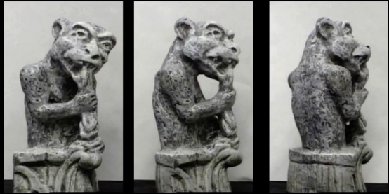
But we have two eyes!

Stereo:

• The image from one eye is a little different than the image from the other eye
• Think of shape from "motion" between two views
• Infer 3D shape of scene from two (multiple) images from different viewpoints

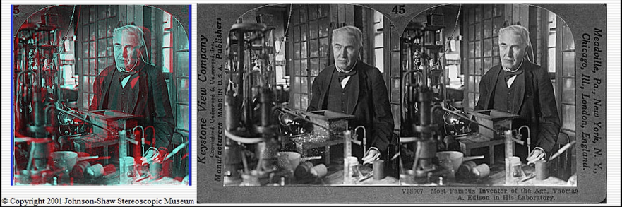
Stereo Photography and Stereo Viewers

Take two pictures of the same subject from slightly different viewpoints and display so that each eye sees only one of the images.

Analygph stereo: put down sort of red and blue imageery and use filters to see each image from an eye

Fig.23: Example of a stereo photo. The image on the left is anaglyph stereo

Stereo Basic Idea

The image below shows an alternation of the two images that slightly differ. Watch lecture for explanation

Fig.24: The basic idea behind stereo. Showin an alternation of the two images

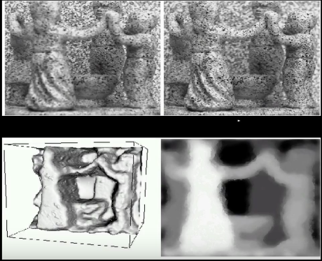
Random Dot Stereograms

Human binuclar fusion is not based upon matching large-scale structure, or any indiviual process of the image. It is acutally based on a low-level process that directly fuses the two images.

Watch the lesson for more explanation

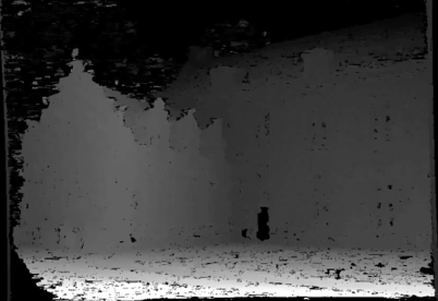
Estimating Depth with Stereo

• Assume we have two cameras, and they're both looking at some scene point, the 3D depth of a point can be recunstruected by figuring out which two points in the two cameras are that point

• Stereo: shape from "motion" between two views. We'll need to consider:
  • Image point correspondences
  • Info on camera pose ("calibration")

Fig.25: Depect stereo setup

Geometry for a simple stereo system

• First, assuming parallel optical axes, known camera parameters (i.e., calibrated cameras) (Figure 26)
• Figure is looking down on the cameras and image plane
• Baseline $\color{blue}{B}$, focal length $\color{blue}{f}$
• Point $\color{blue}{p}$ is distance $\color{blue}{Z}$ in camera coordinate systems
• $\color{blue}{Z}$ is the distance all the way to center of projection (COP) not image plane. Review previous lesson
• Point $\color{blue}{P}$ projects into left and right images.
• Distance is positive in left image and negative in right

Fig.26(a)

Fig.26(b)

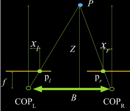
What is the expression for $Z$?

• Similar triangles ($\color{blue}{p_l}$, $\color{blue}{P}$, $\color{blue}{p_r}$) and ($\color{blue}{C_l}$, $\color{blue}{P}$, $\color{blue}{C_r}$)

Fig.26(c): first triangle

Fig.26(d): second triangle

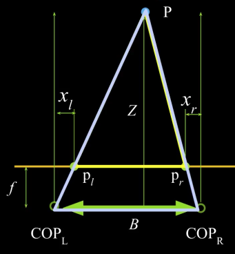
So,

$$\color{blue}{\frac{B - x_l + x_r}{Z-f} = \frac{B}{Z}}$$

$$\color{blue}{\Rightarrow \,\,\,\, Z = f \frac{B}{x_l - x_r}}$$

What happens when disparity ($\color{blue}{x_l - x_r}$) is zero?

• At some point in the scene, the point is projected at the same point in the left and the right images, and thus the depth is infinit. (e.g. the moon)

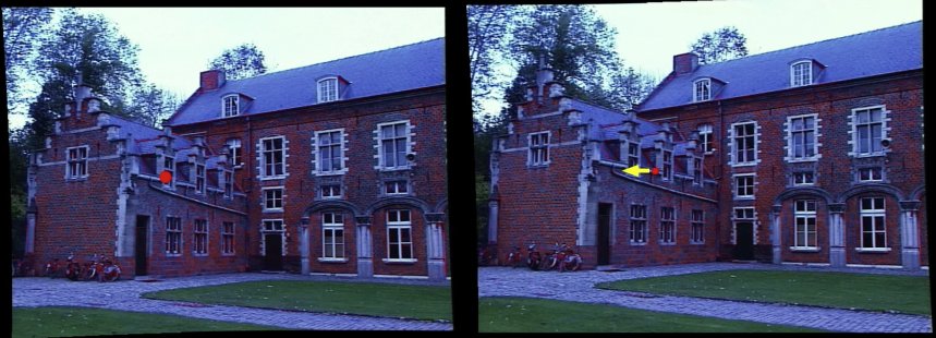
**Quize**

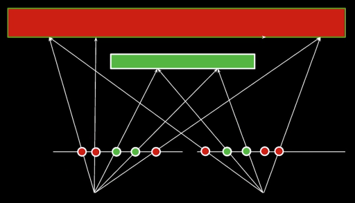
Which image is the left and which is right?

Fig.26(e) quiz

Left is in the left image, and Right in the right one. Because we know that the person is in front of the tree, that means image on the person in the right image should be shifted to the left

Depth from disparity

More on the video

Fig.27(a): example of depth from disparity. Notice the window at the red point to the left image is shifted to the left the right image

Fig.27(b): Disparity map, for every point what is the disparity, the brighter the closer

%matplotlib inline
import numpy as np
import cv2
from matplotlib import pyplot as plt
import PIL
from io import BytesIO
from IPython.display import clear_output, Image as NoteImage, display
def imshow(im,fmt='jpeg'):
    #a = np.uint8(np.clip(im, 0, 255))
    f = BytesIO()
    PIL.Image.fromarray(im).save(f, fmt)
    display(NoteImage(data=f.getvalue()))
def imread(filename):
    img = cv2.imread(filename)
    img = cv2.cvtColor(img, cv2.COLOR_BGR2RGB)
    return img

imgL = cv2.imread('imgs/SuXT483.png',0)
imgR = cv2.imread('imgs/Yeuna9x.png',0)
stereo = cv2.StereoBM_create(numDisparities=16, blockSize=7)
disparity = stereo.compute(imgL,imgR)

fig, ax = plt.subplots(ncols=3)
fig.set_size_inches((15,25))
ax[0].imshow(imgL,'gray')
ax[1].imshow(imgR,'gray')
ax[2].imshow(disparity,'gray')
plt.show()

=====================================

3B - L2 Epipolar geometry

=====================================

Stereo Correspondence Constraints

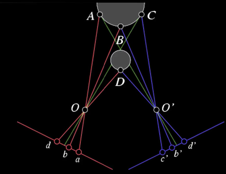
General case, with calibrated cameras

• The two cameras need not have parallel optical axes and image planes
• Cameras can be parallel or converged

Fig.28(a): parallel versus converged cameras

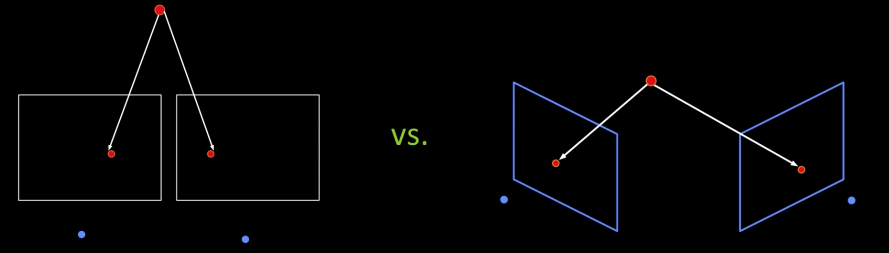
• Remember: in prespective projection, lines project into lines
• So, the line containing the center of projection and the point P in the left image must project to a line in the right image Figure(28 b).

Fig.28(b): parallel versus converged cameras

Terms

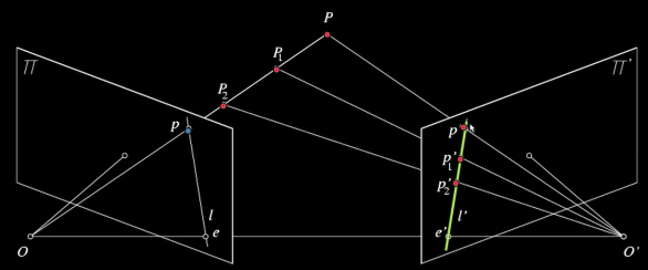
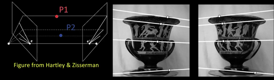
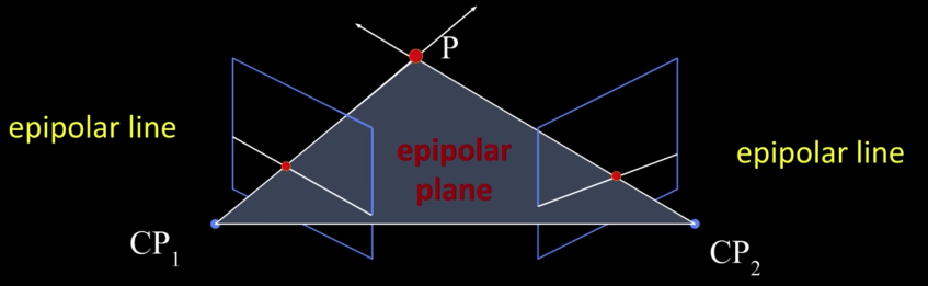
Epipolar constraint

• Geometry of two views constrains where the corresponding pixel for some image point in the first view must occur in the second view.

• Baseline: line joining the camera centers

• Epipolar plane for a given piont: plane containing baseline and world point
• Epipolar line: intersection of epipolar plane with the image plain - come in pairs
• Epipole: point of intersection of baseline with the image plane
  

Fig.29 Epipolar constraint

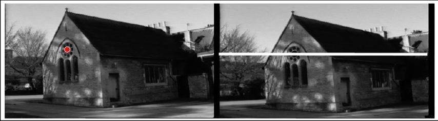
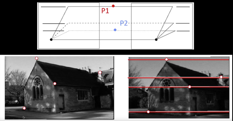
Epipolar Constraint

The epipolar constraint reduces the correspondence problem to a 1D search along an epipolar line.

Fig.30(a): example of searching space along the epipolar line

Fig.30(b): converged vs parallel epipolar line

Converging cameras

Where is the epipole?

Somewhere outside the image but not in the infinity.

Explanation in the lecture

Fig.31 example of epipolar lines in converging cameras

Parallel image planes

Where is the epipole?

At the infinity

Explanation in the lecture

Fig.33 example of epipolar lines in parallel cameras

Quiz

Fig.34 quiz

How do we know that (B) has parallel image planes?

a) The epipolar lines are horizontal
b) The epipolar lines are parallel
c) Because I just said that (B) had parallel image plane

import cv2
import numpy as np
from matplotlib import pyplot as plt


img1 = cv2.imread('imgs/left.jpg',0) #queryimage # left image
img2 = cv2.imread('imgs/right.jpg',0) #trainimage # right image

sift = cv2.xfeatures2d.SIFT_create()

# find the keypoints and descriptors with SIFT
kp1, des1 = sift.detectAndCompute(img1,None)
kp2, des2 = sift.detectAndCompute(img2,None)

# FLANN parameters
FLANN_INDEX_KDTREE = 0
index_params = dict(algorithm = FLANN_INDEX_KDTREE, trees = 5)
search_params = dict(checks=50)

flann = cv2.FlannBasedMatcher(index_params,search_params)
matches = flann.knnMatch(des1,des2,k=2)

good = []
pts1 = []
pts2 = []

# ratio test as per Lowe's paper
for i,(m,n) in enumerate(matches):
    if m.distance < 0.8*n.distance:
        good.append(m)
        pts2.append(kp2[m.trainIdx].pt)
        pts1.append(kp1[m.queryIdx].pt)
        
pts1 = np.int32(pts1)
pts2 = np.int32(pts2)
F, mask = cv2.findFundamentalMat(pts1,pts2,cv2.FM_LMEDS)

# We select only inlier points
pts1 = pts1[mask.ravel()==1]
pts2 = pts2[mask.ravel()==1]

def drawlines(img1,img2,lines,pts1,pts2):
    ''' img1 - image on which we draw the epilines for the points in img2
        lines - corresponding epilines '''
    r,c = img1.shape
    img1 = cv2.cvtColor(img1,cv2.COLOR_GRAY2BGR)
    img2 = cv2.cvtColor(img2,cv2.COLOR_GRAY2BGR)
    for r,pt1,pt2 in zip(lines,pts1,pts2):
        color = tuple(np.random.randint(0,255,3).tolist())
        x0,y0 = map(int, [0, -r[2]/r[1] ])
        x1,y1 = map(int, [c, -(r[2]+r[0]*c)/r[1] ])
        img1 = cv2.line(img1, (x0,y0), (x1,y1), color,1)
        img1 = cv2.circle(img1,tuple(pt1),3,color,-1)
        img2 = cv2.circle(img2,tuple(pt2),3,color,-1)
    return img1,img2

# Find epilines corresponding to points in right image (second image) and
# drawing its lines on left image
lines1 = cv2.computeCorrespondEpilines(pts2.reshape(-1,1,2), 2,F)
lines1 = lines1.reshape(-1,3)
img5,img6 = drawlines(img1,img2,lines1,pts1,pts2)

# Find epilines corresponding to points in left image (first image) and
# drawing its lines on right image
lines2 = cv2.computeCorrespondEpilines(pts1.reshape(-1,1,2), 1,F)
lines2 = lines2.reshape(-1,3)
img3,img4 = drawlines(img2,img1,lines2,pts2,pts1)
fig = plt.gcf()
fig.set_size_inches((20,15))
plt.subplot(121),plt.imshow(img5)
plt.subplot(122),plt.imshow(img3)
plt.show()

😢 Unfortunately, I couldn't find a stereo image for Messi!!!. Messi had a fracture of the radial bone in his right arm yesturday against Sevilla. He will be out for approximately three weeks. 😢

injuredMessi = imread('injuredMessi.jpg')
imshow(injuredMessi)

def display_pair(imgs,titles):
    plt.gray()
    plt.figure(figsize=(20,20))
    
    plt.subplot(121)
    ax = plt.gca()
    ax.xaxis.set_major_locator(plt.NullLocator())
    ax.yaxis.set_major_locator(plt.NullLocator())   
    plt.imshow(imgs[0])
    plt.title(titles[0], size=20)
    if len(imgs)> 1:
        plt.subplot(122)
        plt.imshow(imgs[1])
        plt.title(titles[1], size=20)
    ax = plt.gca()
    ax.xaxis.set_major_locator(plt.NullLocator())
    ax.yaxis.set_major_locator(plt.NullLocator()) 
    fig = plt.gcf()
    fig.tight_layout()
    plt.show()
def resize(image,size):
    return cv2.resize(image, size) 

injuredMessi2 = imread('imgs/injuredMessi2.jpg')
Tsubasa = imread('imgs/Tsubasa.jpg')
injuredMessi2 = resize(injuredMessi2,(Tsubasa.shape[1],Tsubasa.shape[0]))
display_pair([injuredMessi2,Tsubasa],['',''])

<Figure size 432x288 with 0 Axes>

=====================================

3B - L3 Stereo Correspondence

=====================================

For now assume parallel image planes

• Assume parallel (co-planar) image planes
• Assume same focal lengths
• Assume epipolar lines are horizontal
• Assume epipolar lines are at the same $y$ location in the image...

Correspondence problem

Multiple match hypotheses satisfy epipolar constraint, but which is correct?

Fig.35(a): shows the correspondence problem

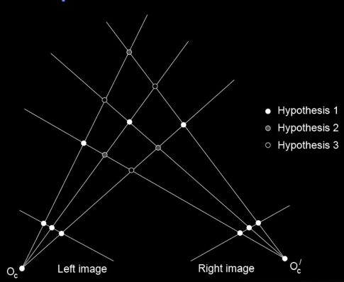
Beyond the hard constraint of epipolar geometry, there are "soft" constraints to help identify corresponding points.

• Similarity: pixel in the right is similar to pixel in the left
• Uniqueness: there is no more than one match of pixel in the left in the right image
• Ordering: if ABC in the left, ABC on the right
• Disparity gradient is limited: the depth doesn't change very quickly

To find matchies in the image pair, we will assume

• Most scene points visible from both views
• Image regions for the matches are similar in appearance

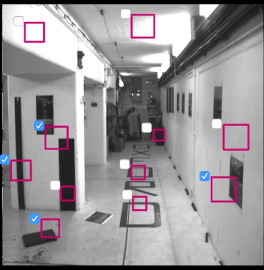
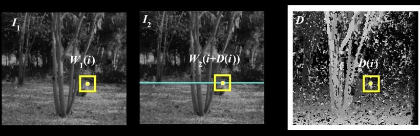
Dense correspondence search

For each pixel/window in the left image:

• Compare with every pixel/window on same epipolar line in right image
• Pick position with minimum match cost( e.g. SSD, normalized correlation)

Fig.35(b) dense correspondence search

def red(im):
    return im[:,:,0]
def green(im):
    return im[:,:,1]
def blue(im):
    return im[:,:,2]
def gray(im):
    return cv2.cvtColor(im, cv2.COLOR_BGR2GRAY)
def square(img,center,size,color=(0,255,0)):
    y,x = center
    leftUpCorner = (x-size,y-size)
    rightDownCorner = (x+size,y+size)
    cv2.rectangle(img,leftUpCorner,rightDownCorner,color,3)
def normalize_img(s):
    start = 0
    end = 255
    width = end - start
    res = (s - s.min())/(s.max() - s.min()) * width + start
    return res.astype(np.uint8)
def line(img,x):
    cv2.line(img,(0,x),(img.shape[1],x),(255,0,0),3) 
def mse(imageA, imageB):
        # the 'Mean Squared Error' between the two images is the
        # sum of the squared difference between the two images;
        # NOTE: the two images must have the same dimension
        err = np.sum((imageA.astype("float") - imageB.astype("float")) ** 2)
        err /= float(imageA.shape[0] * imageA.shape[1])
        # return the MSE, the lower the error, the more "similar"
        # the two images are
        return err

def dense_correspondence_search(point,imgL,imgR,windowSize,disparity_fun=mse):    
    def clip(img,center,windowSize):
        x,y = center
        half = windowSize//2
        return img[x-half:x+half+1,y-half:y+half+1]
    
    queryWindow = clip(imgL,point,windowSize)
    row = point[0]
    disparity = [(col,disparity_fun(queryWindow,clip(imgR,(row,col),windowSize))) 
                 for col in np.arange(windowSize//2,
                                      imgR.shape[1]-imgR.shape[1]%window_size,
                                      windowSize)]
    return np.array(disparity)


def calculate_disparity_img(imgL,imgR,numDisparities=32, blockSize=5):
    stereo = cv2.StereoBM_create(numDisparities=numDisparities, blockSize=blockSize)
    disparity = stereo.compute(imgL,imgR)
    disparity[disparity<0] = 0
    return disparity

point = (200,500)
window_size = 11

redPalaceLeft = imread("imgs/red_palace_l.jpg")
redPalaceRight = imread("imgs/red_palace_r.jpg")

annotatedLeft = redPalaceLeft.copy()
annotatedRight = redPalaceRight.copy()

## Finding disparity
disparity = dense_correspondence_search(point,gray(redPalaceLeft),
                                       gray(redPalaceRight),window_size)
## Finding minimum disparity 
dindex, dvalues = disparity[:,0],disparity[:,1]
minIndex = np.argmin(dvalues)
minY = int(dindex[minIndex])
rightPoint = (point[0],minY)

## Annotating
square(annotatedLeft,point,window_size)
line(annotatedRight,point[0])
square(annotatedRight,rightPoint,window_size)

display_pair([annotatedLeft,annotatedRight],["left","right"])
print("Disparity")
plt.plot(dvalues)

<Figure size 432x288 with 0 Axes>

Disparity

[<matplotlib.lines.Line2D at 0x121f42748>]

Dense Correspondence Problem

point = (500,500)
window_size = 11

redPalaceLeft = imread("imgs/red_palace_l.jpg")
redPalaceRight = imread("imgs/red_palace_r.jpg")

annotatedLeft = redPalaceLeft.copy()
annotatedRight = redPalaceRight.copy()

## Finding disparity
disparity = dense_correspondence_search(point,gray(redPalaceLeft),
                                       gray(redPalaceRight),window_size)
## Finding minimum disparity 
dindex, dvalues = disparity[:,0],disparity[:,1]
minIndex = np.argmin(dvalues)
minY = int(dindex[minIndex])
rightPoint = (point[0],minY)

## Annotating
square(annotatedLeft,point,window_size)
line(annotatedRight,point[0])
square(annotatedRight,rightPoint,window_size)

display_pair([annotatedLeft,annotatedRight],["left","right"])
print("Disparity")
plt.plot(dvalues)

<Figure size 432x288 with 0 Axes>

Disparity

[<matplotlib.lines.Line2D at 0x121693dd8>]

Quiz

Which region are good for dense search?

Fig.36: Quize

Effect of window size

point = (500,500)
window_sizes = [5,7,9,11,13,15,17,19,21]

redPalaceLeft = imread("imgs/red_palace_l.jpg")
redPalaceRight = imread("imgs/red_palace_r.jpg")
annotatedLeft = redPalaceLeft.copy()
annotatedRight = redPalaceRight.copy()

squares = []
disparities = []
for window_size in window_sizes:
    ## Finding disparity
    disparity = dense_correspondence_search(point,gray(redPalaceLeft),
                                           gray(redPalaceRight),window_size)
    ## Finding minimum disparity 
    dindex, dvalues = disparity[:,0],disparity[:,1]
    minIndex = np.argmin(dvalues)
    minY = int(dindex[minIndex])
    rightPoint = (point[0],minY)

    ## Annotating
    square(annotatedLeft,point,window_size)
    line(annotatedRight,point[0])
    square(annotatedRight,rightPoint,window_size)
    
    disparities.append(disparity[:,1])
    
    
display_pair([annotatedLeft,annotatedRight],["left","right"])

fig, axs = plt.subplots(ncols=3,nrows=3)
fig = plt.gcf()
fig.set_size_inches((20,15))
import itertools
index = list(itertools.product(range(3), range(3)))
for c,w,d in zip(range(len(window_sizes)),window_sizes,disparities):
    ax = axs[index[c][0],index[c][1]]
    ax.plot(d)
    ax.set_title("Window size: %d" % w)

<Figure size 432x288 with 0 Axes>

redPalaceLeft = gray(imread("imgs/red_palace_l.jpg"))
redPalaceRight = gray(imread("imgs/red_palace_r.jpg"))
window_sizes = [5,7,9,11,13,15,25,33,41]

disparities = []
for w in window_sizes:
    ## Finding disparity
    disparity = calculate_disparity_img(redPalaceLeft,redPalaceRight,
                                        numDisparities=16,blockSize=w)
    disparities.append(disparity)

display_pair([redPalaceLeft,redPalaceRight],["left","right"])
fig, axs = plt.subplots(ncols=3,nrows=3)
fig = plt.gcf()
fig.set_size_inches((20,15))
import itertools
index = list(itertools.product(range(3), range(3)))
for c,w,d in zip(range(len(window_sizes)),window_sizes,disparities):
    ax = axs[index[c][0],index[c][1]]
    ax.imshow(d,'gray')
    ax.set_title("Window size: %d" % w)

<Figure size 432x288 with 0 Axes>

Occlusion

Uniqueness constraint

No more than one match in right image for every point in left image.

Note the second most right pixel in the right image and the second most left pixel in the left image in the figure below. These pixels are only visible to one image but not the other

Fig.37: Occlusion example

Ordering Constraint

The image below shows an example of a violation of ordering constraints happens because of a narrow occluding surface.

Fig.38: violation of ordering constraints

Stereo Results

Better solutions

Beyond individual correspondences to estimate disparities:

• Optimize correspondence assignments jointly
  • Scanline at a time (DP)
  • Full 2D grid (graph cuts)

Dynamic Programming Formulation

Review the lecture

Coherent stereo on 2D grid- DP

Scanline stereo generates streaking artificats. Can't use dynamic programming to find spatially coherent disparities/ correspondences on a 2D grid

Fig.39(a): artifacts of dynamic programming

What defines a good stereo correspondence?

1. Match quality: Want each pixel to find a good appearance match in the other image
2. Smoothness: of two pixels are adjacent, they should (usually) move about the same amount

Stereo matching as energy minimization

Fig.39(b): energy minimization

Data term $$\color{blue}{E_{data} = \sum_i{(W_1(i) - W_2(i + D(i)))^2}}$$

Smoothness term $$\color{blue}{E_{smooth} = \sum_{neighbors\,\, i,j}\rho(D(i)-D(j))}$$

Total energy $$\color{blue}{E = \alpha\, E_{data}(I_1,I_2,D) + \beta\,E_{smooth}(D)}$$

Middlebury Stereo Vision Page

Better Results and Challenges

• Energy functions of this form can be minimized using graph cuts

Fig.40: results of graph cuts

The below is the results produced by the Implementation of graph cuts

imgL = cv2.imread('imgs/red_palace_l.jpg',0)
imgR = cv2.imread('imgs/red_palace_r.jpg',0)
disparity = cv2.imread('imgs/red_palace_disp.png')


fig, ax = plt.subplots(ncols=2)
fig.set_size_inches((15,25))
ax[0].imshow(imgL,'gray')
ax[0].set_title("Left")
ax[1].imshow(imgR,'gray')
ax[1].set_title("Right")
fig, ax = plt.subplots(ncols=1)
fig.set_size_inches((15,25))
ax.set_title("Disparity Using graph cuts")
ax.imshow(disparity)
plt.show()

=====================================

3C - L1 Extrinsic Camera Parameters

=====================================

Review Model Projection

Projection equations:

• Compute intersection with Perspective Projection of ray from (x,y,z) to COP
• Derived using similar triangles $$\color{blue}{(X,Y,Z) -> (-d\frac{X}{Z},-d\frac{Y}{Z},-d}$$ (assumes normal Z negative - we will change later)
• We get the projection by throwing out the last coordinate: $$\color{blue}{(x',y') = (-d\frac{X}{Z},-d\frac{Y}{Z})}$$
  

Homogeneous coordinates

Perspective Proejction

More above

Geometric Camera Calibration

• We want to use the camera to tell us things about the world
  • So we need the relationship between coordinates in the world and coordinates in the image: geometric camera calibration
• For reference see Forsyth and Ponce, sections 1.2 and 1.3

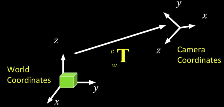
Composed of 2 trnasformation

• From some (arbitraty) world coordinate system to the camera's 3D coordinate system. Extrinsic parameters (or camera pose)
• From the 3D coordinates in the camera frame to the 2D image plane via projection. Intrinsic parameters

Camera Pose

Fig.41: Camera pose

Quiz

How many degrees of freedom are there in specifying the extrinsic parameters?

a) 5
b) 6
c) 3
d) 9

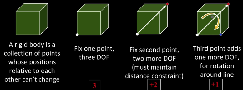
Rigid Body Transformation

Need a way to specify the six degrees-of-freedom of a rigid body why 6?

1. Moving in space
2. Rotating around the vertical and the horizontal axis
3. Rotating around diagonal axis

Fig.42: Rigid Body Transformation

Notation (from F&P)

• Superscript references coordinate frame
• $\color{blue}{p^A}$ is coordinates of P in frame A
• $\color{blue}{p^B}$ is coordinates of P in frame B

$$\color{blue}{p^A = \begin{bmatrix} x^A \\ y^A \\ z^A \end{bmatrix} \Leftrightarrow \overline{OP} = (x^A \cdot \overline{i_A}) + (y^A \cdot \overline{j_A}) + (z^A \cdot \overline{k_A})}$$

Translation Only

$$\color{blue}{p^B = p^A + (O_A)^B}$$

or $$\color{blue}{ p^B = (O_A)^B + p^A}$$

Fig.43: Translation

Using homogeneous coordinates, translation can be expressed as a matrix multiplication.

$$\color{blue}{ p^B = (O_A)^B + p^A}$$

$$\color{blue}{\begin{bmatrix} p^B \\ 1 \end{bmatrix} = \begin{bmatrix} I & (O_A)^B \\ 0^T & 1 \end{bmatrix} \begin{bmatrix} p^A \\ 1 \end{bmatrix}}$$

Rotation

$$\color{blue}{ \overline{OP} = \begin{bmatrix} i_A & j_A & k_A\end{bmatrix} \begin{bmatrix} x^A \\ y^A \\ z^A\end{bmatrix} = \begin{bmatrix} i_B & j_B & k_B\end{bmatrix}\begin{bmatrix} x^B \\ y^B \\ z^B\end{bmatrix} }$$

$$\color{blue}{ p^B = R^B_A\,P^A}$$

$\color{blue}{R^B_A}$: means describing frame A in the coordinate system of frame B

Fig.44: Rotation

What does R look like?

$$\color{blue}{R^B_A = \begin{bmatrix}i_A i_B&j_A i_B&k_A i_B\\i_A j_B&j_A j_B&k_A j_B\\i_A k_B&j_A k_B&k_A k_B \end{bmatrix}}$$
$$\color{blue}{ = \begin{bmatrix}i_A^B & j_A^B & k_A^B \end{bmatrix}}$$
$$\color{blue}{ = \begin{bmatrix}i^{A(T)}_B \\ j^{A(T)}_B \\ k^{A(T)}_B \end{bmatrix}}$$

T is the transpose

Example: Rotation about z axis

Fig.45: Rotation about z axis

What is the rotation matrix?

$$\color{blue}{R_z(\theta) = \begin{bmatrix} cos(\theta) & -sin(\theta) & 0 \\s in(\theta) & cos(\theta) & 0 \\ 0 & 0 & 1 \end{bmatrix}}$$

Combine 3 to get arbitrary rotation

• Euler angles: Z, X', Z''
• Or heading, pitch, roll: world Z, new X, new Y
• Or roll, pitch, and yaw
• Or Azimuth, elevation, roll
• Three basic matrices: order matters, but we'll not focus on that

$$\color{blue}{R_x(\varphi) = \begin{bmatrix} 1 & 0 & 0 \\ 0 & cos(\varphi) & -sin(\varphi) \\ 0 & sin(\varphi) & cos(\varphi) \end{bmatrix}}$$

$$\color{blue}{R_z(\theta) = \begin{bmatrix} cos(\theta) & -sin(\theta) & 0 \\s in(\theta) & cos(\theta) & 0 \\ 0 & 0 & 1 \end{bmatrix}}$$

$$\color{blue}{R_y(\kappa) = \begin{bmatrix} cos(\kappa) 0 & & -sin(\kappa) \\ 0 & 1 & 0 \\s in(\kappa) & 0 & cos(\kappa) \end{bmatrix}}$$

Rotation in homogeneous coordinates

• Using homogeneous coordinates, rotation can be expressed as a matrix multiplication.

$$\color{blue}{ p^B = R^B_A\,P^A}$$

$$\color{blue}{\begin{bmatrix} p^B \\ 1 \end{bmatrix} = \begin{bmatrix} I & O_A^B \\ 0^T & 1 \end{bmatrix} \begin{bmatrix} p^A \\ 1 \end{bmatrix}}$$

Rotation is not commutative

Rigid Transformation

Fig.46: total rigid transformation

$$ \color{blue}{p^B = R_A^Bp^A + (O_A)^B }$$

Unified treatment using homogeneous coordinates:

$$\color{blue}{\begin{bmatrix} p^B \\ 1 \end{bmatrix} = \begin{bmatrix} 1 & O_A^B \\ 0^T & 1 \end{bmatrix}\begin{bmatrix} R_A^B & 1 \\ 0^T & 1 \end{bmatrix} \begin{bmatrix} p^A \\ 1 \end{bmatrix}}$$

$$\color{blue}{ = \begin{bmatrix} R_A^B &O_A^B\\ 0^T & 1 \end{bmatrix}\begin{bmatrix} p^A \\ 1 \end{bmatrix} }$$

And even better:

$$\color{blue}{ \begin{bmatrix} p^B \\ 1 \end{bmatrix} = \begin{bmatrix} R_A^B &O_A^B\\ 0^T & 1 \end{bmatrix}\begin{bmatrix} p^A \\ 1 \end{bmatrix} = T^B_A\begin{bmatrix} p^A \\ 1 \end{bmatrix} }$$

$$\color{blue}{ \begin{bmatrix} p^A \\ 1 \end{bmatrix} = T^A_B\begin{bmatrix} p^B \\ 1 \end{bmatrix} = (T^B_A)^-1\begin{bmatrix} p^B \\ 1 \end{bmatrix}}$$

Translation and Rotation

From frame A to B:

Non-homogeneous ("regular") coordinates:

$$\color{blue}{\overrightarrow{p}^B = R_A^B \overrightarrow{p}^A + \overrightarrow{t^B_A} }$$

$$\color{blue}{\overrightarrow{p}^B = \begin{bmatrix} &&&|\\ &R_A^B&&\overrightarrow{t^B_A}\\&&&|\\0&0&0&1 \end{bmatrix} \begin{bmatrix} x \\ y \\ z\\1 \end{bmatrix} }$$

Homogenous coordinates allows us to write coordinate transforms as a single matrix!

From World to Camera

Non-homogeneous coordinates $$\color{blue}{\overrightarrow{p}^C = R_W^C\,\, \overrightarrow{p}^W + \overrightarrow{t}^C_W }$$

$\color{blue}{\overrightarrow{p}^C}$: Point in the camera frame
$\color{blue}{\overrightarrow{p}^W }$: Point in world frame
$\color{blue}{R_W^C}$: Rotation from world to camera frame
$\color{blue}{\overrightarrow{t}^C_W}$: Translation from world to camera frame

$$\color{blue}{\begin{bmatrix} \\ \overrightarrow{p}^C \\ \\ \\ \end{bmatrix} = \begin{bmatrix} -&-&-&|\\ -&R_W^C&-&\overrightarrow{t^C_W}\\-&-&-&|\\0&0&0&1 \end{bmatrix} \begin{bmatrix} \\ \overrightarrow{p}^W \\ \\ \\ \end{bmatrix} }$$

From world to camera is the extrinsic parameter matrix (4X4)

Quiz

How many degrees of freedom are there in 3X4 extrinsic parameter matrix?

a) 12
b) 6
c) 9
d) 3

Three angles that controls the rotation matrix and three values that controls the translation

Showing Translation

from transforms3d.affines import compose
import numpy as np
P1 = np.array([[0],[0],[0],[1]])
P2 = np.array([[0],[3],[1.5],[1]])
P3 = np.array([[0],[0],[3],[1]])
T = [0, 0, 10] # translations
R = [[1, 0, 0], [0, 1, 0], [0, 0, 1]] # rotation matrix
Z = [1, 1, 1] # zooms
A = compose(T, R, Z)
TP1 = np.matmul(A,P1)
TP2 = np.matmul(A,P2)
TP3 = np.matmul(A,P3)

xdata = [P1[0],P2[0],P3[0],TP1[0],TP2[0],TP3[0]]
ydata = [P1[1],P2[1],P3[1],TP1[1],TP2[1],TP3[1]]
zdata = [P1[2],P2[2],P3[2],TP1[2],TP2[2],TP3[2]]

import matplotlib.pyplot as plt
from mpl_toolkits import mplot3d
fig = plt.figure(figsize=(15,15))

ax = plt.axes(projection='3d')

ax.scatter3D(xdata, ydata, zdata, cmap='Greens');

ax.plot([P1[0][0],P2[0][0]],[P1[1][0],P2[1][0]],zs=[P1[2][0],P2[2][0]],c="red")
ax.plot([P1[0][0],P3[0][0]],[P1[1][0],P3[1][0]],zs=[P1[2][0],P3[2][0]],c="blue")
ax.plot([P2[0][0],P3[0][0]],[P2[1][0],P3[1][0]],zs=[P2[2][0],P3[2][0]],c="green")

ax.plot([TP1[0][0],TP2[0][0]],[TP1[1][0],TP2[1][0]],zs=[TP1[2][0],TP2[2][0]],c="red")
ax.plot([TP1[0][0],TP3[0][0]],[TP1[1][0],TP3[1][0]],zs=[TP1[2][0],TP3[2][0]],c="blue")
ax.plot([TP2[0][0],TP3[0][0]],[TP2[1][0],TP3[1][0]],zs=[TP2[2][0],TP3[2][0]],c="green")




plt.show()

Showing Rotation

from transforms3d.euler import euler2mat, mat2euler
import matplotlib.pyplot as plt
from mpl_toolkits import mplot3d

def plot_square(TP,ax):
    p1 = TP[0].flatten(); p2 = TP[1].flatten(); p3 = TP[2].flatten(); p4 = TP[3].flatten(); 
    ax.plot([p1[0],p2[0]],[p1[1],p2[1]],zs=[p1[2],p2[2]],c="red")
    ax.plot([p2[0],p3[0]],[p2[1],p3[1]],zs=[p2[2],p3[2]],c="blue")
    ax.plot([p3[0],p4[0]],[p3[1],p4[1]],zs=[p3[2],p4[2]],c="green")
    ax.plot([p4[0],p1[0]],[p4[1],p1[1]],zs=[p4[2],p1[2]],c="yellow")

########
x_angle = 0
y_angle = 0
z_angle = 0
R1 = euler2mat(x_angle, y_angle, z_angle, 'sxyz')
x_angle = 0
y_angle = 0
z_angle = -np.pi / 2
R2 = euler2mat(x_angle, y_angle, z_angle, 'sxyz')
x_angle = 0
y_angle = np.pi / 2
z_angle = 0
R3 = euler2mat(x_angle, y_angle, z_angle, 'sxyz')
########

P1 = np.array([[0],[0],[0],[1]])
P2 = np.array([[0],[1],[0],[1]])
P3 = np.array([[0],[1],[1],[1]])
P4 = np.array([[0],[0],[1],[1]])
PS = [P2,P3,P4,P1]
T1 = [0, 0, 0] # No Translations
T2 = [1, 0, 0] # X-Translations
T3 = [0, 1, 0] # Y-Translations
Z = [1, 1, 3] # zooms
   
A1 = compose(T1, R1, Z) # No Rotation
A2 = compose(T1, R2, Z) # Rotation about Z-axis
A3 = compose(T1, R3, Z) # Rotation about Y-axis
A4 = compose(T2, R1, Z) # X-Translation 
A5 = compose(T3, R2, Z) # Y-Translation + Rotation about Z-axis

fig = plt.figure(figsize=(15,15))
ax = plt.axes(projection='3d')

plot_square([np.matmul(A1,p) for p in PS],ax)
plot_square([np.matmul(A2,p) for p in PS],ax)
plot_square([np.matmul(A3,p) for p in PS],ax)
plot_square([np.matmul(A4,p) for p in PS],ax)
plot_square([np.matmul(A5,p) for p in PS],ax)

plt.show()

=====================================

3C - L2 Intrinsic Camera Parameters

=====================================

Ideal intrinsic parameters

Ideal Perspective projection:

$$\color{blue}{u = f\frac{x}{z}}$$
$$\color{blue}{v = f\frac{y}{z}}$$

Fig.47 (a): Ideal perspective projection

Real intrinsic parameters(1)

But "pixels" are in some arbitrary spatial units $$\color{blue}{u = \alpha\frac{x}{z}}$$
$$\color{blue}{v = \alpha\frac{y}{z}}$$

Real intrinsic parameters(2)

Maybe pixels are not square $$\color{blue}{u = \alpha\frac{x}{z}}$$
$$\color{blue}{v = \beta\frac{y}{z}}$$

Real intrinsic parameters(3)

We don't know the origin of our camera pixel coordinates $$\color{blue}{u = \alpha\frac{x}{z} + u_0}$$
$$\color{blue}{v = \beta\frac{y}{z}+v_0}$$

Real intrinsic parameters(4)

May be skew between camera pixel axes $$\color{blue}{v'sine(\theta) = v}$$
$\color{blue}{$u' = u - cos(\theta)v' = u - cot(\theta)v}$$

Fig.47 (b): Real perspective projection

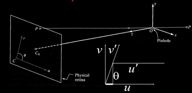
Really ugle intrinsic parameters (4)

$$\color{blue}{u= \alpha\frac{x}{z}-\alpha cot(\theta)\frac{y}{z} + u_0}$$ $$\color{blue}{v = \frac{\beta}{sin(\theta)}\frac{y}{z} + v_0}$$

Improving Intrinsic Parameters

$$\color{blue}{ \begin{bmatrix}z*u \\ z*v \\ z \end{bmatrix} = \begin{bmatrix} \alpha&-\alpha cot(\theta)&u_0&0\\ 0&\frac{\beta}{sin(\theta)}&v_0&0\\0&0&1&0 \end{bmatrix} \begin{bmatrix} x \\ y \\ z\\1 \end{bmatrix} }$$

$$\color{blue}{\overrightarrow{p'} = K \overrightarrow{p}^C }$$

$\color{blue}{\overrightarrow{p'}}$: in homogeneous pixel
$\color{blue}{\overrightarrow{p}^C}$: in camera-based 3D coords
K: Intrinsic matrix

Kinder, gentler intrinsics

• Can use simpler notation for intrinsics, remove last column whihc is zero:

$$\color{blue}{K = \begin{bmatrix}f&s&c_x\\0&af&c_y\\0&0&1\end{bmatrix}}$$

f: focal length
s: skew
a: aspect ratio
$c_x,c_y$: offset

(5 DOF)

• If sqaure pixels, no skew, and optical center is in the center (assume origin in the middle):

$$\color{blue}{K = \begin{bmatrix}f&0&0\\0&f&0\\0&0&1\end{bmatrix} }$$

Quiz

Thhe intrinsics have the following: a focal length, a pixel x size, a pixel y size, two offsets and a skew. That's 6. But we've said there only 5 DOFS. What happened?

a) Because $f$ always multiplies the pixel sizes, those 3 numbers are really only 2 DOFs
b) In modern cameras, the skew is always zero, so we don't count it.
c) In CCDs or CMOS cameras, the aspect is carefully controlled to be 1.0, so it is no longer modeled

Combining Extrinsic and Intrinsic Calibration Parameters

Intrinsic
$$\color{blue}{\overrightarrow{p'} = K \overrightarrow{p}^C }$$
Extrinsic

$$\color{blue}{\begin{bmatrix} \\ \overrightarrow{p}^C \\ \\ \\ \end{bmatrix} = \begin{bmatrix} -&-&-&|\\ -&R_W^C&-&\overrightarrow{t^C_W}\\-&-&-&|\\0&0&0&1 \end{bmatrix} \begin{bmatrix} \\ \overrightarrow{p}^W \\ \\ \\ \end{bmatrix} }$$

$\color{blue}{\overrightarrow{p'}}$ : Pixels
$\color{blue}{\overrightarrow{p^W}}$ : World coordinate
$\color{blue}{\overrightarrow{p}^C}$: Camera 3D coordinates
$\color{blue}{\overrightarrow{p}^W}$: World 3D coordinates
K: 3X3 (no need for the 1 at the bottom of the matrix) or 3X4

$$\color{blue}{\overrightarrow{p'} = K(R_W^C \,\, \overrightarrow{t}_W^C) \overrightarrow{p}^W}$$

$\color{blue}{(R_W^C \,\, \overrightarrow{t}_W^C)}$: 3X4

$$\color{blue}{\overrightarrow{p'} = M \,\, \overrightarrow{p}^W}$$

Other Ways to Write the Same Equation

$$\color{blue}{ \begin{bmatrix} u\\v\\1 \end{bmatrix} \simeq \begin{bmatrix}s*u \\ s*v \\ s \end{bmatrix} = \begin{bmatrix} \cdot & m^T_1 & \cdot &\cdot\\ \cdot & m^T_2& \cdot & \cdot \\\cdot & m^T_3 & \cdot & \cdot\end{bmatrix}\begin{bmatrix} P_x^W \\ P_y^W \\P_z^W \\1\end{bmatrix}}$$

Conversion back from homogeneous coordinates

$$\color{blue}{u = \frac{m_1\cdot \overrightarrow{P}}{m_3\cdot \overrightarrow{P}} }$$ $$\color{blue}{v = \frac{m_2\cdot \overrightarrow{P}}{m_3\cdot \overrightarrow{P}} }$$

$\color{blue}{\simeq}$: projectively similar

Camera Parameters

• A camera (and its matrix) M (or $\color{blue}{\Pi}$) is described by several parameters
  • Translation T of the optical center from the origin of the world coordinates
  • Rotation R of the camera system
  • focal length and aspect (f,a) [or pixel size $(s_x,s_y)$], principle point $\color{blue}{(x'_c,y'_c)}$, and skew (s)
  • blue parameters are called extrinsics, red are intrinsics

$$\color{blue}{ X \simeq \begin{bmatrix} sx\\sy\\s \end{bmatrix} = \begin{bmatrix} * & * & * & * \\ * & * & * & * \\ * & * & * & * \end{bmatrix} \begin{bmatrix} X\\Y\\Z \\ 1 \end{bmatrix} = MX} $$

$$\color{blue}{ M = \begin{bmatrix}f&s&x'_c\\0&af&y'_c\\0&0&1\end{bmatrix} \begin{bmatrix}1&0&0&0\\0&1&0&0\\0&0&1&0\end{bmatrix}\begin{bmatrix} R_{3X3} & 0_{3X1}\\0_{1X3} & 1\end{bmatrix}\begin{bmatrix} I_{3X3} & T_{3X1}\\0_{1X3} & 1\end{bmatrix}} $$

There are 11 DoFs: 5 + 0 + 3 + 3

=====================================

3C - L3 Calibrating cameras

=====================================

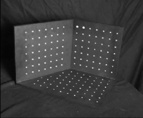
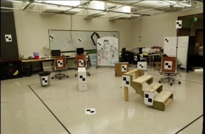
Calibration using known points

Place a known object in the scene

• Identify correspondence between image and scene
• compute mapping from scene to image

Fig.48 (a): Calibration using knonw points

Resectioning

Estimating the camera matrix from known 3D points Projective Camera Matrix

$$\color{blue}{ p = K\begin{bmatrix}R & t \end{bmatrix}P = MP \begin{bmatrix}w*u\\w*v\\w \end{bmatrix} = \begin{bmatrix} m_{11} & m_{12} & m_{13} & m_{14} \\ m_{21} & m_{22} & m_{23} & m_{24} \\ m_{31} & m_{32} & m_{33} & m_{34} \\ m_{41} & m_{42} & m_{43} & m_{44} \end{bmatrix}\begin{bmatrix}X \\Y \\Z \\1 \end{bmatrix}}$$

Fig.48 (a): Calibration using resectioning

Direct linear calibration - homogeneous

$$\color{blue}{\begin{bmatrix} u_i \\ v_i \\ 1 \end{bmatrix} \cong \begin{bmatrix}w*u_i\\w*v_i\\w \end{bmatrix} = \begin{bmatrix} m_{00} & m_{01} & m_{02} & m_{03} \\ m_{10} & m_{11} & m_{12} & m_{13} \\ m_{20} & m_{21} & m_{22} & m_{23} \\ m_{30} & m_{31} & m_{32} & m_{33} \end{bmatrix}\begin{bmatrix}X \\Y^i \\Z^i \\1^i \end{bmatrix}}$$

One pair of equations for each point

$$\color{blue}{ u_i = \frac{m_{00}X_i + m_{01}Y + m_{02}Z + m_{03}}{m_{20}X_i + m_{21}Y + m_{22}Z + m_{23}}}$$

$$\color{blue}{ v_i = \frac{m_{10}X_i + m_{11}Y + m_{12}Z + m_{13}}{m_{20}X_i + m_{21}Y + m_{22}Z + m_{23}}}$$

$$\color{blue}{u_i(m_{20}X_i + m_{21}Y + m_{22}Z + m_{23}) = m_{00}X_i + m_{01}Y + m_{02}Z + m_{03}}$$

$$\color{blue}{ v_i(m_{20}X_i + m_{21}Y + m_{22}Z + m_{23}) = m_{10}X_i + m_{11}Y + m_{12}Z + m_{13}}$$

$$\color{blue}{\begin{bmatrix}X_i & Y_i&Z_i&1&0&0&0&-u_iX_i&-u_iY_i & -u_iZ_i -u_i\\ X_i & Y_i&Z_i&1&0&0&0&-v_iX_i&-v_iY_i & -v_iZ_i -v_i \end{bmatrix}\begin{bmatrix} m_{00}\\ m_{10}\\ m_{02}\\ m_{03}\\ m_{10}\\ m_{11}\\ m_{12}\\ m_{13}\\ m_{20}\\ m_{21}\\ m_{22}\\ m_{23} \end{bmatrix} =\begin{bmatrix} 0 \\ 0\end{bmatrix}}$$

• This is a homogenous set of equations.
• When over constrained, defines a least squares problem - minimize $||Am||$
• Since m is only defined up to scale, solve for unit vector m*
  • Solution: m = eigenvector of $A^TA$ with smallest eigenvalue
  • Works with 6 or more points

The SVD (singular value decomposition) Trick Part1

$$\color{blue}{\begin{bmatrix} X_i & Y_i&Z_i&1&0&0&0&-u_iX_i&-u_iY_i & -u_iZ_i -u_i\\ X_i & Y_i&Z_i&1&0&0&0&-v_iX_i&-v_iY_i & -v_iZ_i -v_i \\ &&&&&.&&&& \\ &&&&&.&&&& \\ &&&&&.&&&& \\ X_n & Y_n&Z_n&1&0&0&0&-u_nX_n&-u_nY_n & -u_nZ_n -u_n\\ X_n & Y_n&Z_n&1&0&0&0&-v_nX_n&-v_nY_n & -v_nZ_n -v_n \end{bmatrix}\begin{bmatrix} m_{00}\\ m_{10}\\ m_{02}\\ m_{03}\\ m_{10}\\ m_{11}\\ m_{12}\\ m_{13}\\ m_{20}\\ m_{21}\\ m_{22}\\ m_{23} \end{bmatrix} =\begin{bmatrix} 0 \\ 0 \\ . \\ . \\ . \\ 0 \\ 0\end{bmatrix}}$$

A: 2n x 12
m: 12
0: 2n

• Find the m that minimizes $\color{blue}{||Am||}$ subject to $\color{blue}{||m|| = 1}$
• Let A = $\color{blue}{UDV^T}$ (singular value decomposition, D diagonal, U and V orthogonal)
• There minimizing $\color{blue}{||UDV^Tm||}$
• But, $\color{blue}{||UDV^Tm||}$ = $\color{blue}{||DV^Tm||}$ and $\color{blue}{||m|| = ||V^Tm||}$
• Thus minimize $\color{blue}{||DV^Tm||}$ subject to $\color{blue}{||v^Tm|| = 1}$
• Let $\color{blue}{y= V^Tm}$. Now minimize $\color{blue}{||Dy||}$ subject to $\color{blue}{||y|| = 1}$
• But D is diagonal, with decreasing values. So $\color{blue}{||Dy||}$ minimum is when $\color{blue}{y = (0,0,0,...,0,1)^T}$
• Since $\color{blue}{y = V^Tm}$, $\color{blue}{m = Vy}$ since $\color{blue}{V}$ orthogonal
• Thus $\color{blue}{m = Vy}$ is the last column in $\color{blue}{V}$
• And, the singular values of A are square roots of the eigenvalues of $\color{blue}{A^T}$ and the columns of V are the eigenvectors. (Show this? Nah...)
  
  
• Recap: Given Am=0, find the eigenvector of $\color{blue}{A^TA}$ with smallest eigenvalue, that's m

from scipy import linalg
m, n = 12, 6
a = np.random.randn(m, n) + 1.j*np.random.randn(m, n)
U, s, Vh = linalg.svd(a)
print(U.shape,  s.shape, Vh.shape)

(12, 12) (6,) (6, 6)

#Reconstruct the original matrix from the decomposition:
sigma = np.zeros((m, n))
for i in range(min(m, n)):
    sigma[i, i] = s[i]
a1 = np.dot(U, np.dot(sigma, Vh))
np.allclose(a, a1)

True

#Alternatively, use full_matrices=False (notice that the shape of U is then (m, n) instead of (m, m)):
U, s, Vh = linalg.svd(a, full_matrices=False)
U.shape, s.shape, Vh.shape

S = np.diag(s)
np.allclose(a, np.dot(U, np.dot(S, Vh)))

True

s2 = linalg.svd(a, compute_uv=False)
np.allclose(s, s2)

True

More References

More explanation and code

Image Compression and SVD

👽 We will borrow the image compression code from the taturial above to see apply it on Messi👽

# from https://github.com/rameshputalapattu/jupyterexplore

from numpy.linalg import svd
from skimage import img_as_ubyte,img_as_float
def compress_svd(image,k):
    """
    Perform svd decomposition and truncated (using k singular values/vectors) reconstruction
    returns
    --------
      reconstructed matrix reconst_matrix, array of singular values s
    """
    U,s,V = svd(image,full_matrices=False)
    reconst_matrix = np.dot(U[:,:k],np.dot(np.diag(s[:k]),V[:k,:]))
   
    return reconst_matrix,s
def compress_show_color_images_reshape(img_name,k):
    """
     compress and display the reconstructed color image using the reshape method 
    """
    image = img_as_float(imread(img_name))
    original_shape = image.shape
    image_reshaped = image.reshape((original_shape[0],original_shape[1]*3))
    image_reconst,_ = compress_svd(image_reshaped,k)
    image_reconst = image_reconst.reshape(original_shape)
    compression_ratio =100.0* (k*(original_shape[0] + 3*original_shape[1])+k)/(original_shape[0]*original_shape[1]*original_shape[2])
    title = "compression ratio={:.2f}".format(compression_ratio)+"%"
    return image_reconst,title

img100,disc100 = compress_show_color_images_reshape("imgs/messi_p2.jpg",100)
img304,disc304  = compress_show_color_images_reshape("imgs/messi_p2.jpg",304)
img20,disc20  = compress_show_color_images_reshape("imgs/messi_p2.jpg",20)
fig, axs = plt.subplots(ncols=3,nrows=1)
fig.set_size_inches((20,5))
axs[0].imshow(img20)
axs[1].imshow(img100)
axs[2].imshow(img304)

axs[0].set_title(disc20)
axs[1].set_title(disc100)
axs[2].set_title(disc304)

Clipping input data to the valid range for imshow with RGB data ([0..1] for floats or [0..255] for integers).
Clipping input data to the valid range for imshow with RGB data ([0..1] for floats or [0..255] for integers).
Clipping input data to the valid range for imshow with RGB data ([0..1] for floats or [0..255] for integers).

Text(0.5,1,'compression ratio=105.62%')

⚽️ Fantástico Leo⚽️

Direct Linear Calibration Inhomogeneous

• Another approach: 1 in lower r.h. corner for 11 d.o.f

$$\color{blue}{\begin{bmatrix} u \\ v \\ 1 \end{bmatrix} \simeq \begin{bmatrix} m_{00} & m_{01} & m_{02} & m_{03} \\ m_{01} & m_{11} & m_{12} & m_{13} \\ m_{01} & m_{21} & m_{22} & 1 \\ \end{bmatrix}\begin{bmatrix}X \\Y \\Z \\1 \end{bmatrix}}$$

$$\color{blue}{ u_i = \frac{m_{00}X_i + m_{01}Y + m_{02}Z + m_{03}}{m_{20}X_i + m_{21}Y + m_{22}Z + 1}}$$

$$\color{blue}{ v_i = \frac{m_{10}X_i + m_{11}Y + m_{12}Z + m_{13}}{m_{20}X_i + m_{21}Y + m_{22}Z + 1}}$$

Dangerous if $m_{23}$ is really (near) zero

Direct Linear Calibration Transformation

Advantages

• Very simple to formulate and solve. Can be done, say on a problem set
• These methods are referred to as "algebraic error" minimization

Disadvantages:

• Doesn't directly tell you the camera parameters
• Approximate: e.g. doesn't model radial distortion
• Hard to impose constraints (e.g. known focal length)
• Mostly: doesn't minimize the right error function

Geometric Error

minimize $E = \sum_{i}d(x'_i, \hat{x}'_i)$

$\hat{x}'_i$: Predicted Image locations

$$min_M \sum_{i}d(x'_i, MX_i)$$

Fig.49: geometric error

"Gold Standard" algorithm (Hartley and Zisserman)

Objective:
Given $n \geq 6$ 3D to 2D point correspondence ${X_i \leftrightarrow x'_i} $, determine the "Maximum Likelihood Estimation" of M

Algorithm:

(i) Linear Solution:
(a) (Optional) Normalization: $\tilde{X}_i = UX_i$ $\tilde{x}_i$ = $Tx_i$
(b) Direct Linear Transformation minimization
(ii) Minimize geometric error: using the linear estimate as a starting point minimize the geometric error:

$min_M \sum_{i}d($ $\tilde{x}_i$$, $$\tilde{M}$$\tilde{X}_i)$ (iii) Denormalization: $M$ = $T^{-1}$$\tilde{M}$U

The pure way

Finding the 3D Camera Center from M

• M encodes all the parameters. So we should be able to find things like the camera center from M

• Slight change in notation. Let: $\color{blue}{M = [Q | b]}$
  M is (3X4) - b is the last column of $\color{blue}{M}$
• The center C is the null-space camera of projection matrix. So if find C such that: $$\color{blue}{MC=0}$$That will be the center

• Proof: Let X be somewhere between any point P and C

$$\color{blue}{X=\lambda P + (1 - \lambda)C}$$

• And the projection: $$\color{blue}{x=MX= \lambda MP + (1 - \lambda)MC}$$

• For any P, all points on PC ray project on image of P, therefor MC must be zero. So the camera center has to be in the null space

The easy way

• Now the easy way. A formula! If $\color{blue}{M = [Q|b]}$ then:

$$\color{blue}{ C=\begin{bmatrix}-Q^{-1}b\\1\end{bmatrix}}$$

Multi Plane Calibration

Fig.50: Multiplane Calibration

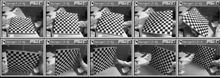
Advantage

• Only requires a plane
• Don't have to know positions/proientations
• Good code available online!
  • OpenCV library
  • Matlab version by Jean-Yves Bouget
  • Zhengyou Zhang's website

import numpy as np
import cv2
import glob

def find_calibration(img,inner_dim=(9,6),crop=False):
# termination criteria
    criteria = (cv2.TERM_CRITERIA_EPS + cv2.TERM_CRITERIA_MAX_ITER, 30, 0.001)

    # prepare object points, like (0,0,0), (1,0,0), (2,0,0) ....,(6,5,0)
    objp = np.zeros((inner_dim[0]*inner_dim[1],3), np.float32)
    objp[:,:2] = np.mgrid[0:inner_dim[0],0:inner_dim[1]].T.reshape(-1,2)

    # Arrays to store object points and image points from all the images.
    objpoints = [] # 3d point in real world space
    imgpoints = [] # 2d points in image plane.
    if type(img) == str:
        img = cv2.imread(img)
    else:
        img = img
    gray_im = cv2.cvtColor(img,cv2.COLOR_BGR2GRAY)
    # Find the chess board corners
    ret, corners = cv2.findChessboardCorners(gray_im, (inner_dim[0],inner_dim[1]),None)
    # If found, add object points, image points (after refining them)
    if ret == True:
        objpoints.append(objp)

        corners2 = cv2.cornerSubPix(gray_im,corners,(11,11),(-1,-1),criteria)
        imgpoints.append(corners2)

        # Draw and display the corners
        imgWithPoints = img.copy()
        imgWithPoints = cv2.drawChessboardCorners(imgWithPoints, (inner_dim[0],inner_dim[1]), corners2,ret)
        imshow(imgWithPoints)
        ret, mtx, dist, rvecs, tvecs = cv2.calibrateCamera(objpoints, imgpoints, gray_im.shape[::-1],None,None)
        h,  w = img.shape[:2]
        newcameramtx, roi=cv2.getOptimalNewCameraMatrix(mtx,dist,(w,h),1,(w,h))
        dst = cv2.undistort(img, mtx, dist, None, newcameramtx)
        if crop:
            #crop the image
            x,y,w,h = roi
            dst = dst[y:y+h, x:x+w]  
        return (img,dst)
    else:
        return (img,img)

img,calibrated = find_calibration("imgs/calib_radial_easy.jpg",(7,6),crop=True)
display_pair([img,calibrated],["Original Image","Calibrated Image"])

<Figure size 432x288 with 0 Axes>

from scipy.ndimage import rotate
# crop = True will fail
img,calibrated = find_calibration("imgs/calib_radial.jpg",(5,5),crop=False)
display_pair([img,calibrated],["Original Image","Calibrated Image"])

<Figure size 432x288 with 0 Axes>

# Lets crop it from the side
from scipy.ndimage import rotate
img = imread("imgs/calib_radial.jpg")
img = img[:-40,80:-120,:]
img,calibrated = find_calibration(img,(9,6),crop=True)
display_pair([img,calibrated],["Original Image","Calibrated Image"])

<Figure size 432x288 with 0 Axes>

🤴 From chapter 2, lets blend Messi with a chessboard image and see if we can calibrate the image 🤴

def resize(image,size):
    return cv2.resize(image, size) 
def multiply(image,factor):
    return np.uint8(np.clip(factor*image, 0, 255))
def blend(img1,img2,factor):
    return multiply(img1,factor)+multiply(img2,1-factor)

chess = imread("imgs/calib_radial.jpg")
chess = chess[:-20,80:-120,:]
messi = resize(imread("imgs/messi_p.jpg"),(chess.shape[1],chess.shape[0]))
bl = blend(messi,chess,0.4)
img,calibrated = find_calibration(bl,crop=True)
display_pair([img,calibrated],["Original Image","Calibrated Image"])

<Figure size 432x288 with 0 Axes>

messi = resize(imread("imgs/messi_p2.jpg"),(chess.shape[1],chess.shape[0]))
bl = blend(messi,chess,0.2)
imshow(gray(bl))
img,calibrated = find_calibration(bl,crop=True)
display_pair([img,calibrated],["Original Image","Calibrated Image"])

<Figure size 432x288 with 0 Axes>

😄Awesome😄

🤦‍ Yesturday, Lionel Messi scored twice but Barca slump to thrilling 4-3 defeat against Real Betis 🤦‍

👑Today, Lionel Messi was awarded La Liga best player and top goalscorer for the past season. Moreover, La Liga president Javier Tebas has proposed naming an award for the Spanish top flight's MVP after Lionel Messi. 👑

=====================================

3D-L1 Image to image projections

=====================================

2D Transformation

Fig.51: Transformation

Translation $$\color{blue}{x' = x + \overrightarrow{t}}$$ $$\color{blue}{x' =\begin{bmatrix}I & \overrightarrow{t}\end{bmatrix}\bar{x}}$$ $$\color{blue}{\bar{x}' = \begin{bmatrix}I & \overrightarrow{t}\\0^T&1\end{bmatrix}\bar{x}}$$ See above for example code

Projective Transformation

• Projective transformations: for 2D images it's a 3x3 matrix applied to homogenous coordinates

$$\color{blue}{\begin{bmatrix}x'\\y'\\w'\end{bmatrix} = \begin{bmatrix}a&b&c\\d&e&f\\g&h&i\end{bmatrix}\begin{bmatrix}x\\y\\w\end{bmatrix}}$$

• Translation

$$\color{blue}{\begin{bmatrix}x'\\y'\\1\end{bmatrix} = \begin{bmatrix}1&0&t_x\\0&1&t_y\\0&0&1\end{bmatrix}\begin{bmatrix}x\\y\\1\end{bmatrix}}$$

• Preserves:
  • Lengths/Areas
  • Angles
  • Orientation
  • Lines

---

• Euclidean (Rigid body)

$$\color{blue}{\begin{bmatrix}x'\\y'\\1\end{bmatrix} = \begin{bmatrix}cos(\theta)&-sin(\theta)&t_x\\sin(\theta)&cos(\theta)&t_y\\0&0&1\end{bmatrix}\begin{bmatrix}x\\y\\1\end{bmatrix}}$$

• Preserves:
  • Lenghts/Areas
  • Angles
  • Lines

---

• Similarity (trans, rot, scale) transform

$$\color{blue}{\begin{bmatrix}x'\\y'\\1\end{bmatrix} = \begin{bmatrix}\alpha cos(\theta)&-\alpha sin(\theta)&t_x\\\alpha sin(\theta)&\alpha cos(\theta)&t_y\\0&0&1\end{bmatrix}\begin{bmatrix}x\\y\\1\end{bmatrix}}$$

• Preserves:
  • Lenghts/Areas
  • Angles
  • Lines

---

• Affine transform

$$\color{blue}{\begin{bmatrix}x'\\y'\\1\end{bmatrix} = \begin{bmatrix}a&b&c\\d&e&f\\0&0&1\end{bmatrix}\begin{bmatrix}x\\y\\w\end{bmatrix}}$$

• Preserves:
  • Parallel Lines
  • Ratio of Areas
  • Lines

---

Projective Trasformation

• Remember, these are homogeneous coordinates

$$\color{blue}{\begin{bmatrix}x'\\y'\\1\end{bmatrix} \cong \begin{bmatrix}sx'\\sy'\\s\end{bmatrix} = \begin{bmatrix}a&b&c\\d&e&f\\g&h&i\end{bmatrix}\begin{bmatrix}x\\y\\1\end{bmatrix}}$$

• General projective trasform (or Homography)

$$\color{blue}{\begin{bmatrix}x'\\y'\\1\end{bmatrix} \cong \begin{bmatrix}wx'\\wy'\\w\end{bmatrix} = \begin{bmatrix}a&b&c\\d&e&f\\g&h&i\end{bmatrix}\begin{bmatrix}x\\y\\1\end{bmatrix}}$$

• Preserves:
  • Lines
  • Also cross ratios

Quiz 1:

Suppose I told you the transform from image A to image B is a translation. How many pairs of corresponding points would you need to know to compute transformation?

a) 3
b) 1
c) 2
d) 4

Quiz 2:

Suppose I told you the transform from image A to image B is a affine. How many pairs of corresponding points would you need to know to compute transformation?

a) 3
b) 1
c) 2
d) 4

Quiz 3:

Suppose I told you the transform from image A to image B is a homography. How many pairs of corresponding points would you need to know to compute transformation?

a) 3
b) 1
c) 2
d) 4

LETS DO MESSI STUFF

import numpy as np
transform = lambda tx,ty,theta,alpha,p: np.matmul(
    np.array([[alpha*np.cos(theta),-1*alpha*np.sin(theta),tx],
              [alpha*np.sin(theta),alpha*np.cos(theta),ty],
              [0,0,1]]),p.T)

# translation
x,y = 10, 10
p1 = np.array([x,y,1])
p2 = transform(0,0,np.pi/2,1,p1)
print(p1,p2)

[10 10  1] [-10.  10.   1.]

import scipy
messi = imread("imgs/messi_training.jpg")

# translation
b_p = np.array([[455,486,1],[530,480,1],
               [450,560,1],[530,560,1]])
tx,ty = 0, -250
theta = 0
alpha = 1
t_p = transform(tx,ty,theta,alpha,b_p).astype(np.int).T
messi[t_p[0][0]:t_p[1][0],t_p[0][1]:t_p[3][1]] = messi[b_p[0][0]:b_p[1][0],b_p[0][1]:b_p[3][1]]
imshow(messi)

🤔 Without Looking, Where is the added ball 🤔

# rotate
messi_2 = messi[0:530,400:650]
imshow(messi_2)
rot = scipy.ndimage.rotate(messi_2,-50,cval=255)
imshow(rot)

😴 Rotation is not soo cool 😴

=====================================

3D-L2 Homographies and mosaics

=====================================

Projective plane

What is the geometric intuition of using homogeneous coordinates?

• A point in the image is a ray in projective space

Fig.52: Projective plane

Each point (x,y) on the plane (at z=1) is represented by a ray (sx,sy,s)

All points on the ray are equivalent:

$$\color{blue}{(x,y,1) \cong (sx,sy,s)}$$

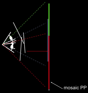
Image reprojection

Basic question:

How to relate to images from the same camera center?

How to map a pixel from projective plane PP1 to PP2?

Answer:

• Cast a ray through each pixel in PP1
• Draw the pixel where that ray intersects PP2

Observation:

• Rather than thinking of this as a 3D reprojection, think of it as a 2D image wrap from one image (plane) to another (plane)
  

Fig.53: Image reprojection

Application: Simple mosaics

Basic Procedure

• Take a sequence of images from the same position
  • Rotate the camera about its optical center
• Compute transformation between second image and first
• Transform the second image to overlap with the first
• Blend the two together to creae a mosaic
• (If there are more images, repeat)

## Code from: https://www.pyimagesearch.com/2016/01/11/opencv-panorama-stitching/
import numpy as np
import imutils
import cv2

class Stitcher:
    def __init__(self):
        # determine if we are using OpenCV v3.X
        self.isv3 = imutils.is_cv3()

    def stitch(self, images, ratio=0.75, reprojThresh=4.0,
        showMatches=False):
        # unpack the images, then detect keypoints and extract
        # local invariant descriptors from them
        (imageB, imageA) = images
        (kpsA, featuresA) = self.detectAndDescribe(imageA)
        (kpsB, featuresB) = self.detectAndDescribe(imageB)

        # match features between the two images
        M = self.matchKeypoints(kpsA, kpsB,
            featuresA, featuresB, ratio, reprojThresh)

        # if the match is None, then there aren't enough matched
        # keypoints to create a panorama
        if M is None:
            return None

        # otherwise, apply a perspective warp to stitch the images
        # together
        (matches, H, status) = M
        result = cv2.warpPerspective(imageA, H,
            (imageA.shape[1] + imageB.shape[1], imageA.shape[0]))
        result[0:imageB.shape[0], 0:imageB.shape[1]] = imageB

        # check to see if the keypoint matches should be visualized
        if showMatches:
            vis = self.drawMatches(imageA, imageB, kpsA, kpsB, matches,
                status)

            # return a tuple of the stitched image and the
            # visualization
            return (result, vis)

        # return the stitched image
        return result

    def detectAndDescribe(self, image):
        # convert the image to grayscale
        gray = cv2.cvtColor(image, cv2.COLOR_BGR2GRAY)

        # check to see if we are using OpenCV 3.X
        if self.isv3:
            # detect and extract features from the image
            descriptor = cv2.xfeatures2d.SIFT_create()
            (kps, features) = descriptor.detectAndCompute(image, None)

        # otherwise, we are using OpenCV 2.4.X
        else:
            # detect keypoints in the image
            detector = cv2.FeatureDetector_create("SIFT")
            kps = detector.detect(gray)

            # extract features from the image
            extractor = cv2.DescriptorExtractor_create("SIFT")
            (kps, features) = extractor.compute(gray, kps)

        # convert the keypoints from KeyPoint objects to NumPy
        # arrays
        kps = np.float32([kp.pt for kp in kps])

        # return a tuple of keypoints and features
        return (kps, features)

    def matchKeypoints(self, kpsA, kpsB, featuresA, featuresB,
        ratio, reprojThresh):
        # compute the raw matches and initialize the list of actual
        # matches
        matcher = cv2.DescriptorMatcher_create("BruteForce")
        rawMatches = matcher.knnMatch(featuresA, featuresB, 2)
        matches = []

        # loop over the raw matches
        for m in rawMatches:
            # ensure the distance is within a certain ratio of each
            # other (i.e. Lowe's ratio test)
            if len(m) == 2 and m[0].distance < m[1].distance * ratio:
                matches.append((m[0].trainIdx, m[0].queryIdx))

        # computing a homography requires at least 4 matches
        if len(matches) > 4:
            # construct the two sets of points
            ptsA = np.float32([kpsA[i] for (_, i) in matches])
            ptsB = np.float32([kpsB[i] for (i, _) in matches])

            # compute the homography between the two sets of points
            (H, status) = cv2.findHomography(ptsA, ptsB, cv2.RANSAC,
                reprojThresh)

            # return the matches along with the homograpy matrix
            # and status of each matched point
            return (matches, H, status)

        # otherwise, no homograpy could be computed
        return None

    def drawMatches(self, imageA, imageB, kpsA, kpsB, matches, status):
        # initialize the output visualization image
        (hA, wA) = imageA.shape[:2]
        (hB, wB) = imageB.shape[:2]
        vis = np.zeros((max(hA, hB), wA + wB, 3), dtype="uint8")
        vis[0:hA, 0:wA] = imageA
        vis[0:hB, wA:] = imageB

        # loop over the matches
        for ((trainIdx, queryIdx), s) in zip(matches, status):
            # only process the match if the keypoint was successfully
            # matched
            if s == 1:
                # draw the match
                ptA = (int(kpsA[queryIdx][0]), int(kpsA[queryIdx][1]))
                ptB = (int(kpsB[trainIdx][0]) + wA, int(kpsB[trainIdx][1]))
                cv2.line(vis, ptA, ptB, (0, 255, 0), 1)

        # return the visualization
        return vis

import cv2
imageA = cv2.imread("imgs/sedona_left_01.png")
imageB = cv2.imread("imgs/sedona_right_01.png")
imageA = imutils.resize(imageA, width=400)
imageB = imutils.resize(imageB, width=400)

# stitch the images together to create a panorama
stitcher = Stitcher()
(result, vis) = stitcher.stitch([imageA, imageB], showMatches=True)

# show the images
display_pair([imageA,imageB],["Image A","Image B"])
imshow(vis)
imshow(result)

<Figure size 432x288 with 0 Axes>

Natural Geometry

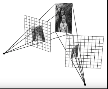
Image reprojection

The mosaic has a natural interpretation in 3D:

• The images are reprojected onto a common plane
• The mosaic is formed on this plane

Warning: This model only holds for angular views up to 180. Beyond that need to use sequence that "bends the rays" or map onto a different surface, say, a cylinder

Fig.54: Mosaic

Mosaics:

Obtain a wider angle view by combining multiple images all of which are taken from the same camera center

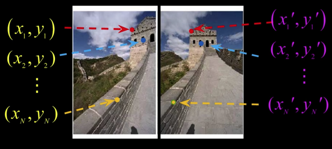
Homography

Assume we have detected corresponding points as in the image below, we have to solve for the equation:

$$\color{blue}{p' = Hp}$$ $$\color{blue}{\begin{bmatrix}wx'\\wy'\\w\end{bmatrix} = \begin{bmatrix}a&b&c\\d&e&f\\g&h&i\end{bmatrix}\begin{bmatrix}x\\y\\1\end{bmatrix}}$$

Fig.55 (a): corresponding points

Solving for homographies - non-homogeneous

Since 8 unknowns, can set scale factor $\color{blue}{i=1$}
Set up a system of linear equations $\color{blue}{Ah = b} where vector of unknowns

$$\color{blue}{h=[a,b,c,d,e,f,g,h]^T}$$

Need at least 4 points for 8 eqs, but more the better...
Solve for h by $\color{blue}{min||Ah-b||^2}$ using least-squares

Solving for homographies - homogeneous

Just like we did for extrinsics, multiply through, and divide out by w
Gives tow homogeneous equations per point.
Solve using SVD just like before. This is the cool way

Apply the Homography

Fig.56(a): Applying homography

Mosaics for Video Coding

• Convert masked images into a background sprite for "content-based coding"

Fig.56(b): Mosaics for Video Coding

**Anyone is welcome to write code example for this in the cell below**

Quiz

We said that the transformation between two images taken from the same center of projection is a homography H. How many pairs of corresponding points do I need to compute H?

a) 6
b) 4
c) 3
d) 8

Homographies and 3D Planes

• Suppose the 3D points are on a plane:

$$\color{blue}{AX + bY = cZ + d = 0}$$

$$\color{blue}{\begin{bmatrix} u \\ v \\ 1 \end{bmatrix} \simeq \begin{bmatrix} m_{00} & m_{01} & m_{02} & m_{03} \\ m_{10} & m_{11} & m_{12} & m_{13} \\ m_{20} & m_{21} & m_{22} & m_{23} \\ \end{bmatrix}\begin{bmatrix}X \\Y \\\frac{aX + bY + d}{-c} \\1 \end{bmatrix}}$$

• So, can put the Z coefficients into the others

$$\color{blue}{\begin{bmatrix} u \\ v \\ 1 \end{bmatrix} \simeq \begin{bmatrix} m'_{00} & m'_{01} & 0 & m'_{03} \\ m'_{10} & m'_{11} & 0 & m'_{13} \\ m'_{20} & m'_{21} & 0 & m'_{23} \\ \end{bmatrix}\begin{bmatrix}X \\Y \\\frac{aX + bY + d}{-c} \\1 \end{bmatrix}}$$

• So, that is 3X3 (3 nonzeros columns), and that is why it is Homography

Image reprojection

• Mapping between planes is a homography
• Whether a plane in the world to the image or between image planes

Fig.57: Image reprojection

## One image of a 3D plane can be aligned with another 
## image of the same plane using Homography

# Read source image.
im_src = imread('imgs/book2.jpg')
# Four corners of the book in source image
pts_src = np.array([[141, 131], [480, 159], [493, 630],[64, 601]])
# Read destination image.
im_dst = imread('imgs/book1.jpg')
# Four corners of the book in destination image.
pts_dst = np.array([[318, 256],[534, 372],[316, 670],[73, 473]])
 
# Calculate Homography
h, status = cv2.findHomography(pts_src, pts_dst)
     
# Warp source image to destination based on homography
im_out = cv2.warpPerspective(im_src, h, (im_dst.shape[1],im_dst.shape[0]))
     
# Display images
display_pair([im_src,im_dst],["Source Image","Destination Image"])
imshow(im_out)

<Figure size 432x288 with 0 Axes>

Image Rectification

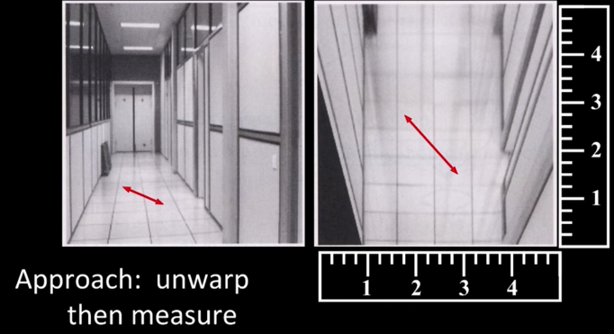
Fig.58(a): Example of rectification

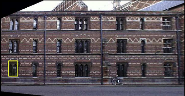
If there is a planar rectangular grid in the scene, you can map it onto a rectangular grid in the image....

Fig.58(b): Measurements on planes

Football Example

Fig.59: Football Example

Forward Warping

Image warping

Given a coordinate trasform and a source image $\color{blue}{f(x,y)}$, how do we compute a transformed image $\color{blue}{g(x',y')}$?

Forward Warping

Send each pixel $\color{blue}{f(x,y)}$ to its corresponding location $\color{blue}{(x',y') T(x,y)}$ in the second image

Fig.60: Forward warping

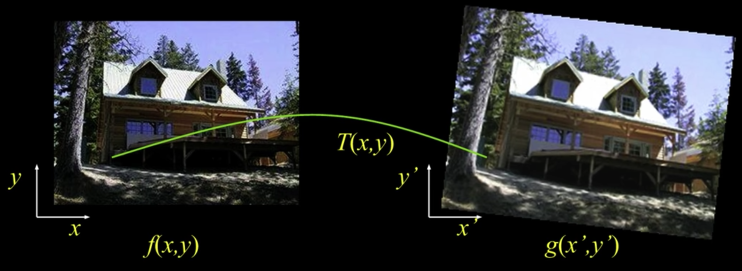
Inverse Warping

Given each pixel $\color{blue}{g(x',y')}$ from its corresponding location $\color{blue}{(x,y) = T^-1(x',y')}$ in the first image

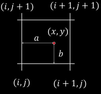
Bilinear interpolation

$$\color{blue}{f(x,y) = (1-a)(1-b)\,\,\,\,\,\, f[i,j]}$$ $$\color{blue}{+\,a(1-b)\,\,\, \,\,\, f[i+1,j]}$$ $$\color{blue}{+\,ab\,\,\,\,\,\, f[i+1,j+1]}$$ $$\color{blue}{+\,(1-a)b\,\,\,\,\,\, f[i,j+1]}$$

Fig.61: Bilinear interpolation

## https://scipython.com/book/chapter-8-scipy/examples/two-dimensional-interpolation-with-scipyinterpolategriddata/

import numpy as np
from scipy.interpolate import griddata
import matplotlib.pyplot as plt

x = np.linspace(-1,1,100)
y =  np.linspace(-1,1,100)
X, Y = np.meshgrid(x,y)

def f(x, y):
    s = np.hypot(x, y)
    phi = np.arctan2(y, x)
    tau = s + s*(1-s)/5 * np.sin(6*phi) 
    return 5*(1-tau) + tau

T = f(X, Y)
# Choose npts random point from the discrete domain of our model function
npts = 400
px, py = np.random.choice(x, npts), np.random.choice(y, npts)

fig, ax = plt.subplots(nrows=2, ncols=2)
# Plot the model function and the randomly selected sample points
ax[0,0].contourf(X, Y, T,cmap='rainbow')
ax[0,0].scatter(px, py, c='k', alpha=0.2, marker='.')
ax[0,0].set_title('Sample points on f(X,Y)')
fig.set_size_inches((15,15))
# Interpolate using three different methods and plot
for i, method in enumerate(('nearest', 'linear', 'cubic')):
    Ti = griddata((px, py), f(px,py), (X, Y), method=method)
    r, c = (i+1) // 2, (i+1) % 2
    ax[r,c].contourf(X, Y, Ti,cmap='rainbow')
    ax[r,c].set_title('method = {}'.format(method))

plt.show()

=====================================

3D-L3 Projective geometry

=====================================

The projective plane

What is the geometric intuition of using homogeneous coordinates?

• A point in the image is a ray in projective space
• Each point (x,y) on the plane (at z=1) is represented by a ray (sx, sy, s)

All points on the ray are equivalent

$$\color{blue}{(x,y,1) \cong (sx,sy,s)}$$

Fig.62: Projective plane

Homogeneous coordinates

2D points:

$$\color{blue}{p = \begin{bmatrix}x\\y\end{bmatrix} ---> p' = \begin{bmatrix}x\\y\\1\end{bmatrix}--->p' = \begin{bmatrix}x'\\y'\\w'\end{bmatrix} --->p= \begin{bmatrix}\frac{x'}{w'}\\\frac{y'}{w'}\end{bmatrix}}$$

2D Lines: ax + by + c = 0

$$\color{blue}{\begin{bmatrix}a&b&c\end{bmatrix}\begin{bmatrix}x\\y\\1\end{bmatrix}=0}$$ $$\color{blue}{l = \begin{bmatrix}a&b&c\end{bmatrix} \Rightarrow \begin{bmatrix}n_x&n_y&-d\end{bmatrix}}$$

Point and Line Duality

What does a line in the image correspond to in projective space?

A line is a plane of rays through origin define by the normal $$\color{blue}{l = (a,b,c)}$$

All rays (x,y,z) satisfying: $$\color{blue}{ax + by + cz = 0}$$

$$\color{blue}{\begin{bmatrix}a&b&c\end{bmatrix}\begin{bmatrix}x\\y\\1\end{bmatrix}=0}$$

A line is also represented as a homogeneous vector

• A line l is a homogeneous 3-vector
• It is $\perp$ to every point (ray) p on the line $\color{blue}{l^Tp=0}$

Fig.63: Projective Lines

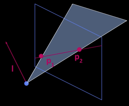
What is the line l spanned by rais $p_1$ and $p_2$?</font>

since $p_1$ is $\perp$ to $p_1$ and $p_2$

$\color{blue}{\Rightarrow}$ $\color{blue}{l = p_1 x p_2}$

What is the interection of two lines $\color{blue}{l_1}$ and $\color{blue}{l_2}$?</font>

since $p$ is $\color{blue}{\perp}$ to $l_1$ and $l_2$ $\color{blue}{\implies}$ $p = l_1xl_2$

Points and lines are dual in projective space

• Given any formula, can switch the meanings of points and lines to get another formula

Homogeneous coordinates

Line joining two points:

$$\color{blue}{p_1 = \begin{bmatrix}x_1&y_1&1\end{bmatrix}}$$ $$\color{blue}{p_2 = \begin{bmatrix}x_2&y_2&1\end{bmatrix}}$$ $$\color{blue}{l = p_1xp_2}$$

Fig.64 (a): Two points

Intersection between two lines:

$$\color{blue}{a_1x - b_1y + c_1 = 0}$$ $$\color{blue}{a_2x - b_2y + c_2 = 0}$$

Fig.64 (b): Two lines

$$\color{blue}{l_1 = \begin{bmatrix}a_1&b_1&c_1\end{bmatrix}}$$ $$\color{blue}{l_2 = \begin{bmatrix}a_2&b_2&c_2\end{bmatrix}}$$ $$\color{blue}{p_{12} = l_1xl_2}$$

Quiz

How can I tell whether a point p is on a line L in an image?
a) Check if p X L is zero
b) Check if $p \cdot L$ is zero
c) Check if the magnitude of the sum is greater than 1

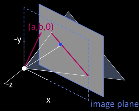
Ideal points and lines

Ideal point ("point at infinity")

$\color{blue}{p \cong (x,y,0)}$ parallel to image plane, has infinit image coordinates

Corresponds to a line in the image (finite coordinates)

- goes through image origin (principle point)

Fig.65: Ideal line

3D projective geometry

• These concepts generalize naturally to 3D
• Recall the equation of a plane: $$\color{blue}{aX + bY + cZ + d = 0}$$
• Homogeneous coordinates
  • Projective 3D points have four coords: $\color{blue}{p = (wX,wY,wZ,w)}$
• Duality
  • A plane N is also represented by a 4-vector
    $\color{blue}{N = (a,b,c,d)}$
  • Points and planes are dual in 3D: $\color{blue}{N^Tp = 0}$
• Projective transformations:
  • Represented by 4X4 matrices T: $\color{blue}{P' = TP}$

=====================================

3D-L4 Essential Matrix

=====================================

Stereo correspondence

Motivating the problem: stereo

• Given two views of a scene (two cameras not necessarily having parallel optical axes) what is the relationship between the location of a scene point in one image and its location in the other?

Stereo Correspondence

Find pairs of points that correspond to same scene point

Fig.66: Stereo Correspondence

Epoipolar Constraint reduces correspondence propblem to 1D search along conjugate epipolar lines

Baseline: line joining the camera centers

Epipolar plane: plane containing baseline and world point

Epipole: point of intersection of baseline with image plane

More above

Stereo Geometry

Stereo geometry, with calibrated cameras

Fig.67: calibrated cameras, assuming T and R is known

Assuming T and R are known $$X'_c = RX_c+T$$

Aside 1

Reminder of cross product

Vector cross product takes two vectors and returns a third vector that's perpendicular to both inputs

$$\color{blue}{\overrightarrow{a}\times \overrightarrow{b} = \overrightarrow{c}}$$

Here c is perpendicular to both a and b, i.e. the dot product = 0

$$\color{blue}{\overrightarrow{a}\cdot \overrightarrow{c} = 0}$$ $$\color{blue}{\overrightarrow{b}\cdot \overrightarrow{c} = 0}$$

Also AxA = 0 for all A

From Geometry to Algebra

Fig.67: calibrated cameras, assuming T and R is known

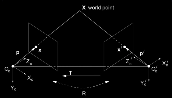
Assuming T and R are known $$\color{blue}{X' = RX+T}$$ $$\color{blue}{T\times X' = T\times RX+T\times T}$$

$\color{blue}{T \times X'}$: Normal to the plane

$$\color{blue}{T\times X' = T\times RX}$$

$$\color{blue}{\implies X' \cdot (T\times X') = X' \cdot(T\times RX)}$$

$$0 = X' \cdot(T\times RX)$$

Aside 2: Matrix form of cross product

$$\color{blue}{\overrightarrow{a}\times \overrightarrow{b} = \begin{bmatrix}0&-a_3&a_2\\a_3&0&-a_1\\-a_2&a_1&0\end{bmatrix}\begin{bmatrix}b_1\\b_2\\b_3\end{bmatrix} = \overrightarrow{c}}$$

We will define a new operator:

$$\color{blue}{[a_x] = \begin{bmatrix}0&-a_3&a_2\\a_3&0&-a_1\\-a_2&a_1&0\end{bmatrix} }$$

So the notation: $$\color{blue}{\overrightarrow{a}\times \overrightarrow{b} = [\overrightarrow{a}_x]\overrightarrow{b}}$$

Essential matrix

$$\color{blue}{0 = X' \cdot(T\times RX)}$$ $$\color{blue}{0 = X' \cdot([T_x]\times RX)}$$

let $\color{blue}{E = [T_x]R}$ $$\color{blue}{X'^TEX = 0}$$

$\color{blue}{E}$ is called the "essential matrix"

More on the lecture

Quiz

That's fine for some convereged cameras. But what if the image planes are parallel. What happens?

a) That is a degenereate case.
b) That's fine. R is just the identity and the math works
c) I have no idea

Essential Matrix Example

Fig.78: Parallel Cameras

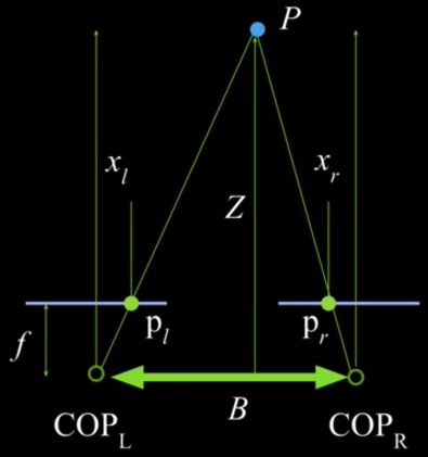
$$\color{blue}{R = I}$$ $$\color{blue}{T = [-B,0,0]^T}$$ $$\color{blue}{E = [T_x]R = \begin{bmatrix}0&0&0\\0&0&B\\0&-B&0\end{bmatrix}}$$

$$\color{blue}{p'^TEp = 0}$$

$$\color{blue}{p = [X,Y,Z] = [\frac{Zx}{f},\frac{Zy}{f},Z]}$$

$$\color{blue}{p' = [X,Y,Z] = [\frac{Zx'}{f},\frac{Zy'}{f},Z]}$$

$$\color{blue}{\begin{bmatrix}x'&y'&f\end{bmatrix}\begin{bmatrix}0&0&0\\0&0&B\\0&-B&0\end{bmatrix}\begin{bmatrix}x\\y\\f\end{bmatrix}=0}$$

$$\color{blue}{\begin{bmatrix}x'&y'&f\end{bmatrix}\begin{bmatrix}0\\Bf\\-By\end{bmatrix}=0}$$

$$\color{blue}{Bfy' = Bfy \implies y' = y}$$

Given a known point $\color{blue}{(x,y)}$ in the original image, this is a line in the $\color{blue}{(x',y')}$ image

import matplotlib.pyplot as plt
from mpl_toolkits import mplot3d
import numpy as np
def plot_square(TP,ax):
    p1 = TP[0].flatten(); p2 = TP[1].flatten(); p3 = TP[2].flatten(); p4 = TP[3].flatten(); 
    ax.plot([p1[0],p2[0]],[p1[1],p2[1]],zs=[p1[2],p2[2]],c="blue")
    ax.plot([p2[0],p3[0]],[p2[1],p3[1]],zs=[p2[2],p3[2]],c="blue")
    ax.plot([p3[0],p4[0]],[p3[1],p4[1]],zs=[p3[2],p4[2]],c="blue")
    ax.plot([p4[0],p1[0]],[p4[1],p1[1]],zs=[p4[2],p1[2]],c="blue")

def create_image_plane(camera,focalLength,fv):
    hfv = fv/2.0
    P1 = np.array([camera[0]-hfv,camera[1]+hfv,camera[2]+focalLength,1])
    P2 = np.array([camera[0]+hfv,camera[1]+hfv,camera[2]+focalLength,1])
    P3 = np.array([camera[0]+hfv,camera[1]-hfv,camera[2]+focalLength,1])
    P4 = np.array([camera[0]-hfv,camera[1]-hfv,camera[2]+focalLength,1])
    return np.array([P2,P3,P4,P1])

def plane_ray_intersection(plane,p1,p2):
    from sympy import Point3D, Plane, Line, Polygon
    point1 = Point3D(plane[0][0], plane[0][1], plane[0][2])
    point2 = Point3D(plane[1][0], plane[1][1], plane[1][2])
    point3 = Point3D(plane[2][0], plane[2][1], plane[2][2])
    point4 = Point3D(plane[3][0], plane[3][1], plane[3][2])
    
    planeL = Plane(point1,point2, point3)
    planeR = Plane(point2,point3, point4)
    line = Line(Point3D(p1[0],p1[1],p1[2]),Point3D(p2[0],p2[1],p2[2]))
    
    inter1 = planeL.intersection(line)
    inter2 = planeR.intersection(line)

    if len(inter1)>0:
        return inter1[0]
    if len(inter2):
        return inter2[0]

    return None



fig = plt.figure(figsize=(10,10))
ax = plt.axes(projection='3d')

## Camera 1
fv = 3
focalLength = 3
camera1 = (0.5,0.5,0.5,1)
iplane1 = create_image_plane(camera1,focalLength,fv)
ax.scatter(camera1[0],camera1[1],camera1[2])
plot_square(iplane1,ax)

## Camera 2
vx = -5;vy = 0;vz = 0
T = np.array([[1,0,0,vx],[0,1,0,vy],[0,0,1,vz]])
camera2 = np.matmul(camera1,T.T)
ax.scatter(camera2[0],camera2[1],camera2[2])
iplane2 = create_image_plane(camera2,focalLength,fv)
plot_square(iplane2,ax)

P = np.array([-2,0.5,10])
ax.scatter(P[0],P[1],P[2])

ax.plot([P[0],camera1[0]],[P[1],camera1[1]],zs=[P[2],camera1[2]],c="red")
ax.plot([P[0],camera2[0]],[P[1],camera2[1]],zs=[P[2],camera2[2]],c="yellow")


ip1 = plane_ray_intersection(iplane1,camera1,P)
ip2 = plane_ray_intersection(iplane2,camera2,P)
print(ip1)
print(ip2)

ax.scatter(ip1[0], ip1[1], ip1[2])
ax.scatter(ip2[0], ip2[1], ip2[2])

Point3D(-11/38, 1/2, 7/2)
Point3D(-141/38, 1/2, 7/2)

<mpl_toolkits.mplot3d.art3d.Path3DCollection at 0x11a8e35f8>

Anyone is welcomed to implement the convereged cameras ones

=====================================

3D-L5 Fundamental matrix

=====================================

Weak Calibration

Main idea:

• Estimate epipolar geometry from a (redundant) set of point correspondences between two uncalibrated cameras

$$\color{blue}{\begin{bmatrix}wx_{im}\\wy_{im}\\w\end{bmatrix} = K_{int}\Phi_{ext} \begin{bmatrix}X_w\\Y_{w}\\Z_w\\1\end{bmatrix}}$$

$$\color{blue}{\Phi_{ext} = \begin{bmatrix} r_{11}&r_{12}&r_{13}&-R_1\ ^tT\\ r_{21}&r_{22}&r_{23}&-R_2\ ^tT\\ r_{31}&r_{32}&r_{33}&-R_3\ ^tT \end{bmatrix}}$$

The rs are the rotation matrix and the RTs are the transformed translation matrix

$$\color{blue}{ K_{int} = \begin{bmatrix} \frac{-f}{s_x} & 0 & o_x\\ 0 & \frac{-f}{s_y} & o_y\\ 0&0&1 \end{bmatrix}}$$

Note: invertible, scale x and y, assumes no skew

$$\color{blue}{p_im = K_{int}\Phi_{ext}P_w}$$

But

$$\color{blue}{\Phi_{ext}P_w=p_c}$$

$\color{blue}{p_c}$: is the 3D point but in the camera frame

$$\color{blue}{p_{im} = K_{int}p_c}$$

Uncalibrated Case

For a given camera: $\color{blue}{\,\,\,p_{im} = K_{int}P_c}$

And since invertible: $\color{blue}{\,\,\,p_{c} = K^{-1}_{int}P_{im}}$

Here $\color{blue}{p_{c}}$ is in terms of the ray. In other words, we only can know the ray that point to the $\color{blue}{P_{im}}$ not a particular point

So, for two cameras (left and right):

$$\color{blue}{p_{c,left} = K^{-1}_{int,left}P_{im,left}}$$
$$\color{blue}{p_{c,right} = K^{-1}_{int,right}P_{im,right}}$$

From before, the essential matrix E:

$$\color{blue}{p_{c,right}\ ^TEp_{c,left}=0}$$

We know it is uncalibrated, but we know their exists an essential matrix. So, we can rewrite

$$\color{blue}{(K^{-1}_{int,right}p_{im,right})^T\,E(K^{-1}_{int,left}p_{im,left}) = 0}$$

Matrix Multiplication

We can regroup:

$$\color{blue}{p^T_{im,right}((K^{-1}_{int,right})^T\,EK^{-1}_{int,left})p_{im,left} = 0}$$
$\color{blue}{(K^{-1}_{int,right})^T\,EK^{-1}_{int,left}}$ is the Fundamental matrix: F

$$\color{blue}{p^T_{im,right}Fp_{im,left} = 0}$$

or

$$\color{blue}{p^TFp'=0}$$

Properties of the Fundamental Matrix

Fig.79 Epipolar constraint

$p^T$Fp'=0
$p^T$ l = 0
l = Fp' is the epipolar line in the p image associated with p'
l' = $F^T$p is the epipolar line in the p image associated with p

description in the lecture

Properties of the Fundamental Matrix (2)

Suppose p' was on the epipolar line, in the prime image for every point p in the original image. This could happen if

$$\color{blue}{Fp' = 0}$$

and $$\color{blue}{F^tp = 0}$$

Epipoles found by solving one of the previous two equations

Properties of the Fundamental Matrix (3)

F is singular (mapping from homogeneous 2-D point to 1-D family so rank 2 - more later)

Fundamental matrix

• Relates pixel coordinates in the two views

• More general form than essential matrix

  • We remove the need to know intrinsic parameters

• If we estimate fundamental matrix from correspondences in pixel coordinates, can reconstruct epipolar geometry without intrinsic or extrinsic parameters

Fig.80: corresponding points and corresponding epipolar lines

Finding the Fundamental Matrix

Fig.81: a camera moving forward and showing the epipole in the intersection between the epipolar lines

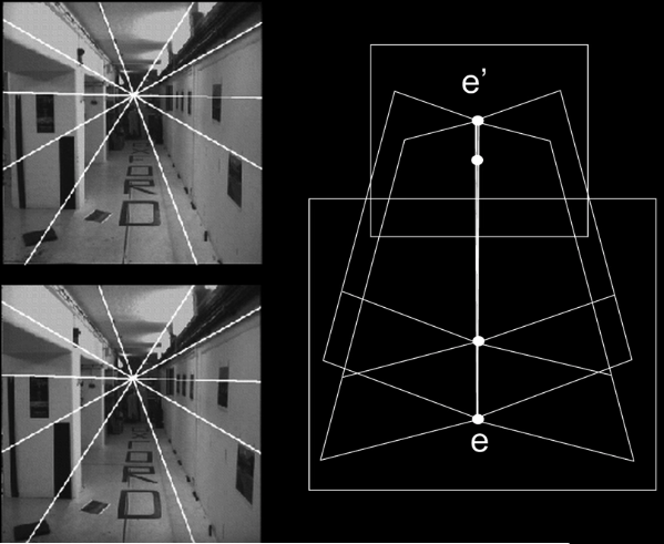
Computing F from correspondences

Each point correspondence generates one constraint on F

$$\color{blue}{P^T_{im,right} F p_{im,left} = 0}$$

$$\color{blue}{\begin{bmatrix}u'&v'&1\end{bmatrix}\begin{bmatrix} f_{11}&f_{12}&f_{13}\\ f_{21}&f_{22}&f_{23}\\ f_{31}&f_{32}&f_{33} \end{bmatrix}\begin{bmatrix}u&v&1\end{bmatrix} = 0}$$

$$\color{blue}{ \begin{bmatrix}u'_1u_1&u'_1v_1&u'_1&v'_1u_1&v'_1v_1 &v'_1&u_1&v_1&1\end{bmatrix} \begin{bmatrix}f_{11}\\f_{12}\\f_{13}\\f_{21}\\f_{22}\\f_{23}\\f_{31}\\f_{32}\\f_{33}\end{bmatrix} }$$

Collect N of these

$$\color{blue}{ \begin{bmatrix} u'_1u_1&u'_1v_1&u'_1&v'_1u_1&v'_1v_1 &v'_1&u_1&v_1&1\\ .&.&.&.&.&.&.&.&\\ .&.&.&.&.&.&.&.&\\ .&.&.&.&.&.&.&.&\\ u'_nu_n&u'_nv_n&u'_n&v'_nu_n&v'_nv_n &v'_n&u_n&v_n&1 \end{bmatrix} \begin{bmatrix}f_{11}\\f_{12}\\f_{13}\\f_{21}\\f_{22}\\f_{23}\\f_{31}\\f_{32}\\f_{33}\end{bmatrix} }$$

The infamous Eight Point Algorithm

From Wikipedia:

The eight-point algorithm is an algorithm used in computer vision to estimate the essential matrix or the fundamental matrix related to a stereo camera pair from a set of corresponding image points. It was introduced by Christopher Longuet-Higgins in 1981 for the case of the essential matrix. In theory, this algorithm can be used also for the fundamental matrix, but in practice the normalized eight-point algorithm, described by Richard Hartley in 1997, is better suited for this case.

The Algorithm from PSU:

• Construct the m x 9 matrix A
• Find the SVD of A: A = UDVT
• The entries of F are the components of the column of V corresponding to the least s.v.

If we use the eight point algorithm to solve for the fundamental matrix and thus find the equations for the epipolar lines for the previous image, we will get something as messy as the one below

Fig.82: finding epipole using eight point algorithm

Rank of F

• Assume w know the homography $\color{blue}{H_\pi}$ that maps from Left to RIght (Full 3X3) $$\color{blue}{p' = H_\pi P}$$
• Let line l' be the epipolar line corresponding to p goes through epipole e'

$$\color{blue}{l' = e'\times p' }$$ $$= e'\times H_\pi p $$ $$\color{blue}{= [e']_\times H_\pi p}$$

But l' is the epipolar line for p
$\color{blue}{l' = Fp}$

So.....

Rank of F is rank of $[e']_\times = 2$

Fig.83: Rank of F

Fix the Linear Solution

• Use SVD or other method to do linear computation for F
• Decompose F using SVD (not the same SVD) $$\color{blue}{F=UDV^T}$$
• Set the last singular value to zero:

$$\color{blue}{D= \begin{bmatrix}r&0&0\\0&s&0\\0&0&t\end{bmatrix}\implies \hat{D} = \begin{bmatrix}r&0&0\\0&s&0\\0&0&0\end{bmatrix} }$$

• Estimate new F from the new $\hat{D}$ $$\color{blue}{\hat{F} = U\hat{D}V^T}$$

Fig.84: Epipole after fixing the linear solution

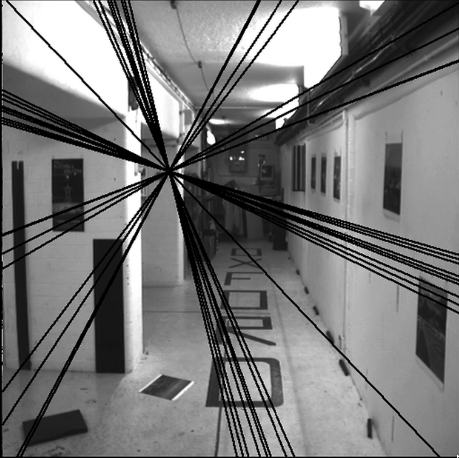
## Code stolen from previous sections above

%matplotlib inline
import cv2
import numpy as np
from matplotlib import pyplot as plt


img1 = cv2.imread('imgs/left.jpg',0) #queryimage # left image
img2 = cv2.imread('imgs/right.jpg',0) #trainimage # right image

sift = cv2.xfeatures2d.SIFT_create()

# find the keypoints and descriptors with SIFT
kp1, des1 = sift.detectAndCompute(img1,None)
kp2, des2 = sift.detectAndCompute(img2,None)

# FLANN parameters
FLANN_INDEX_KDTREE = 0
index_params = dict(algorithm = FLANN_INDEX_KDTREE, trees = 5)
search_params = dict(checks=50)

flann = cv2.FlannBasedMatcher(index_params,search_params)
matches = flann.knnMatch(des1,des2,k=2)

good = []
pts1 = []
pts2 = []

# ratio test as per Lowe's paper
for i,(m,n) in enumerate(matches):
    if m.distance < 0.8*n.distance:
        good.append(m)
        pts2.append(kp2[m.trainIdx].pt)
        pts1.append(kp1[m.queryIdx].pt)
        
pts1 = np.int32(pts1)
pts2 = np.int32(pts2)
F, mask = cv2.findFundamentalMat(pts1,pts2,cv2.FM_LMEDS)

# We select only inlier points
pts1 = pts1[mask.ravel()==1]
pts2 = pts2[mask.ravel()==1]

def drawlines(img1,img2,lines,pts1,pts2):
    ''' img1 - image on which we draw the epilines for the points in img2
        lines - corresponding epilines '''
    r,c = img1.shape
    img1 = cv2.cvtColor(img1,cv2.COLOR_GRAY2BGR)
    img2 = cv2.cvtColor(img2,cv2.COLOR_GRAY2BGR)
    for r,pt1,pt2 in zip(lines,pts1,pts2):
        color = tuple(np.random.randint(0,255,3).tolist())
        x0,y0 = map(int, [0, -r[2]/r[1] ])
        x1,y1 = map(int, [c, -(r[2]+r[0]*c)/r[1] ])
        img1 = cv2.line(img1, (x0,y0), (x1,y1), color,1)
        img1 = cv2.circle(img1,tuple(pt1),3,color,-1)
        img2 = cv2.circle(img2,tuple(pt2),3,color,-1)
    return img1,img2

# Find epilines corresponding to points in right image (second image) and
# drawing its lines on left image
lines1 = cv2.computeCorrespondEpilines(pts2.reshape(-1,1,2), 2,F)
lines1 = lines1.reshape(-1,3)
img5,img6 = drawlines(img1,img2,lines1,pts1,pts2)

# Find epilines corresponding to points in left image (first image) and
# drawing its lines on right image
lines2 = cv2.computeCorrespondEpilines(pts1.reshape(-1,1,2), 1,F)
lines2 = lines2.reshape(-1,3)
img3,img4 = drawlines(img2,img1,lines2,pts2,pts1)
fig = plt.gcf()
fig.set_size_inches((20,15))
plt.subplot(121),plt.imshow(img5)
plt.subplot(122),plt.imshow(img3)
plt.show()

Stero Image Rectification

• Reproject image planes onto a common plane parallel to the line between optical centers - each a homography
• Pixel motion is horizontal after this transformation
• C. Loop and Z. Zhang. Computing Rectifying Homographies for Stereo Vision. IEEE Conf. Computer Vision and Pattern Recognition, 1999

Fig.85: Image Rectification

Applications

Photo Synth

Fig.86 (a): Photo Synth

3D from multiple images

Fig.86 (b): 3D from multiple images

"""
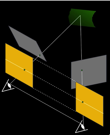
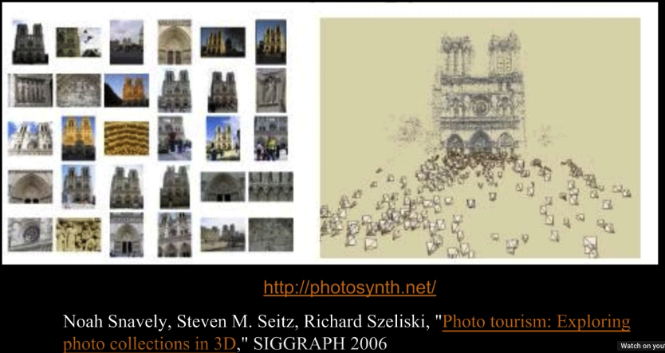
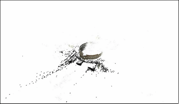
Anyone is welcomed to put code here for the previous 
concepts. I am too busy reading "The bleak house" and 
"The way of kings" :)
"""

Summary

• For 2-views, there is a geometric relationship that defines the relation between rays in one view to rays in the other - epipolar geometry

• These relationships can be captured algebraically as well:

  • Calibrated - Essential matrix
  • Uncalibrated - Fundamental matrix
• This relation can be estimated from point correspondences