import cv2 as cv
import matplotlib.pyplot as plt
import numpy as np
from mpl_toolkits.mplot3d import Axes3D
from IPython.display import clear_output, Image as NoteImage, display
import PIL
from io import BytesIO
from scipy.ndimage.filters import gaussian_filter
def red(im):
return im[:,:,0]
def green(im):
return im[:,:,1]
def blue(im):
return im[:,:,2]
def gray(im):
return cv.cvtColor(im, cv.COLOR_BGR2GRAY)
def plot_row(grayim,index):
y = grayim[index,:]
x = np.arange(len(y))
plt.plot(x,y)
plt.show()
def plot_3d(img):
w,h = img.shape
fig = plt.figure(figsize=(8, 3))
ax1 = fig.add_subplot(111, projection='3d')
_x = np.arange(w)
_y = np.arange(h)
for x in _x:
ax1.plot([x]*h,_y,img[x,:])
%matplotlib notebook
def imshow(im,fmt='jpeg'):
#a = np.uint8(np.clip(im, 0, 255))
f = BytesIO()
PIL.Image.fromarray(im).save(f, fmt)
display(NoteImage(data=f.getvalue()))
def imsave(im,filename,fmt='jpeg'):
#a = np.uint8(np.clip(im, 0, 255))
PIL.Image.fromarray(im).save(filename, fmt)
def imread(filename):
img = cv.imread(filename)
img = cv.cvtColor(img, cv.COLOR_BGR2RGB)
return img
messi = cv.imread("messi.jpg")
messi = cv.cvtColor(messi, cv.COLOR_BGR2RGB)
ball = messi[280:340, 330:390]
messi[273:333, 100:160] = ball
print ("Normal")
imshow(messi)
print ("Additave Inverse")
imshow(255-messi)
print ("Multiply 0.5")
imshow(np.uint8(np.clip(0.5*messi, 0, 255)))


messigreen = green(messi)
messigreen.shape
#plot_row(messigreen,10)
x = np.array([messigreen[139:140,210:270].flatten()]*40)
print("additave inverse")
imshow(255-messigreen)
print("red")
imshow(red(messi))
print("green")
imshow(green(messi))
print("blue")
imshow(blue(messi))
#plot_3d(messigreen[139:140,210:270])


messi2 = cv.imread("messi2.jpg")
messi2 = cv.cvtColor(messi2, cv.COLOR_BGR2RGB)
imshow(messi)
imshow(messi2)

def resize(image,size):
return cv.resize(image, size)
def multiply(image,factor):
return np.uint8(np.clip(factor*image, 0, 255))
messi2 = resize(messi2,(messi.shape[1],messi.shape[0]))
imshow(messi)
imshow(messi2)

print ("Average Image")
messic = multiply(green(messi),0.5)+multiply(green(messi2),0.5)
imshow(messic)

def blend(img1,img2,factor):
return multiply(img1,factor)+multiply(img2,1-factor)
imshow(blend(green(messi),green(messi2),0.35))

Noise
Noise in Image is another function that is combined with the original function to get a new guess what- function
- Salt and pepper noise: random occuences of black and white pixels
- Impulse noise: random occurrences of white pixels
- Gaussian noise: variations in intensity drawn from a Gaussian normal distribution
def gnoise(img,mu,sigma):
noise = np.random.normal(mu, sigma, img.shape)
return np.uint8(img + noise)
print("Gaussian noise")
gausi = gnoise(green(messi),0,8)
imshow(gausi)

# you can also use gaussian filter function from scipy.
from scipy.ndimage import gaussian_filter
blurred = gaussian_filter(messi[:,:,2], sigma=1)
imshow(blurred)

def add_salt_and_pepper(gb, prob):
'''Adds "Salt & Pepper" noise to an image.
gb: should be one-channel image with pixels in [0, 1] range
prob: probability (threshold) that controls level of noise'''
rnd = np.random.rand(gb.shape[0], gb.shape[1])
noisy = gb.copy()
noisy[rnd < prob] = 0
noisy[rnd > 1 - prob] = 1
return np.uint8(noisy*255)
salty = add_salt_and_pepper(green(messi/255.0),0.01)
imshow(salty)

def plot_two(img1,img2,index):
f, (ax1, ax2) = plt.subplots(1, 2)
y = img1[index,:]
x = np.arange(len(y))
ax1.plot(x,y)
y = img2[index,:]
ax2.plot(x, y)
def plot_raw(img1,index):
f, (ax1) = plt.subplots(1, 1)
y = img1[index,:]
x = np.arange(len(y))
ax1.plot(x,y)
def plot_images(imgs, index=None):
rows = len(imgs)
f, axes = plt.subplots(nrows=rows, ncols=1)
for i, img in enumerate(imgs):
y = img[index or 0, :]
x = np.arange(len(y))
axes[i].plot(x,y)
plot_images([green(messi),gausi, blurred], 30)

Difference of images
messid = green(messi) - green(messi2)
imshow(messid)

Brighter area shows where the two images differ more
messid = green(messi2) - green(messi)
imshow(messid)

Oreder matters. But we are interested in the magnitude of the difference not the signed
### messid = abs(green(messi2) - green(messi))
### Te previous will overflow. Instead we use the following
def abs_diff(img1,img2):
return np.uint8(abs(np.int16(img1)- np.int16(img2)))
messid = abs_diff(green(messi2),green(messi))
messid2 = abs_diff(green(messi),green(messi2))
imshow(messid)
imshow(messid2)

%matplotlib inline
def draw_raw(img,index,mag=10):
fig, ax = plt.subplots()
#ax.set_axis_off()
ax.margins(0,0)
#ax.xaxis.set_major_locator(plt.NullLocator())
#ax.yaxis.set_major_locator(plt.NullLocator())
x = np.array([img[index,:]]*mag)
im = ax.imshow(x,cmap="gray")
fig.tight_layout()
draw_raw(messid,300)
plot_raw(messid,300)


Removing noise
Take the average of the pixels around each pixel
Averaging Assumotions
- The true value of pixels are similar to the true value of pixels nearby
- The noise added to each pixel is done independently
Weighted Moving Average
- Can add weights to our moving average
Weights [1,1,1,1,1,]/5
None-uniform weights [1,4,6,4,1]/16
plot_raw(gausi,100)

def moving_average(a, n=3) :
ret = np.cumsum(a, dtype=float)
ret[n:] = ret[n:] - ret[:-n]
return ret[n - 1:] / n
raw100 = gausi[100,:]
cleaned = moving_average(raw100,5)
plt.plot(np.arange(len(cleaned)),cleaned)

def weighted_moving_average(a,weights=np.array([1,4,6,4,1])):
s = sum(weights)
n = len(weights)
h = n//2
ret = [np.dot(a[i-h:i+h+1],weights)//s for i in range(h,len(a)-h)]
return ret
w_cleaned = weighted_moving_average(raw100)
plt.plot(np.arange(len(w_cleaned)),w_cleaned)

plt.plot(np.arange(len(w_cleaned)),w_cleaned,label="Weighted Average")
#plt.plot(np.arange(len(cleaned[5:-5])),cleaned[5:-5],label="Average")
plt.plot(np.arange(len(green(messi)[100,:][5:-5])),green(messi)[100,:][5:-5],label="Original")
plt.legend()

plt.plot(np.arange(len(cleaned)),cleaned,label="Average")
plt.plot(np.arange(len(green(messi)[100,:])),green(messi)[100,:],label="Original")
plt.legend()

Moving average in 2D
def moving_average_2d(a, n=3) :
w,h = a.shape
m = n*n
half = n//2
x = np.copy(a)
for i in range(half,w-half):
for j in range(half,h-half):
s = round(sum(a[i-half:i+half+1,j-half:j+half+1].flatten()))
x[i,j] = s/float(m)
return x
cleaned = moving_average_2d(gausi,3)
imshow(gausi)
imshow(cleaned)

Using Scipy, we can get the same results
mode : str or sequence, optional
The mode parameter determines how the input array is extended when the filter overlaps a border. By passing a sequence of modes with length equal to the number of dimensions of the input array, different modes can be specified along each axis. Default value is ‘reflect’. The valid values and their behavior is as follows:
reflect (d c b a | a b c d | d c b a) The input is extended by reflecting about the edge of the last pixel.
constant (k k k k | a b c d | k k k k) The input is extended by filling all values beyond the edge with the same constant value, defined by the cval parameter.
nearest (a a a a | a b c d | d d d d) The input is extended by replicating the last pixel.
mirror (d c b | a b c d | c b a) The input is extended by reflecting about the center of the last pixel.
wrap (a b c d | a b c d | a b c d) The input is extended by wrapping around to the opposite edge.
from scipy.ndimage import uniform_filter
cleaned = uniform_filter(gausi, size=3, mode='constant')
imshow(cleaned)

Using Convolve
from scipy.ndimage import convolve
kernal = np.ones((3,3))/9
cleaned = convolve(gausi, kernal, mode='constant')
imshow(cleaned)

Using Correlation
from scipy.ndimage import correlate
kernal = np.array([[0.05,0.2,0.05],[0.1,0.2,0.1],[0.05,0.2,0.05]])
cleaned = correlate(gausi, kernal, mode='constant')
imshow(cleaned)

To blur a single pixel into a "blurry" spot, we would need to need to filter the spot with
a. 3x3 square of uniform weights
b. 11x11 square of uniform weights would be better since it's bigger
c. Something that looks like a blurry spot-higher values in the middle, falling off to the edges (C)
Example
# Nearest neighboring pixels have the most influence
kernal = np.array([[1,2,1],[2,4,2],[1,2,1]])/16.0
print (kernal)
Circularly symmetric fuzzy blob
Smooting kernel proportional to: $$e^{(-\frac{x^2 + y^2}{2\sigma^2})}$$
from scipy.ndimage import gaussian_filter
cleaned = gaussian_filter(gausi, sigma=2)
imshow(cleaned)

Gaussian filters
variance ($\sigma^2$) or standard deviation ($\sigma$) detrmines extent of smoothing
The smoother one will work better. The bigger the size the better it is
import matplotlib.pyplot as plt
from mpl_toolkits.mplot3d import Axes3D
import numpy as np
from scipy.stats import multivariate_normal
def plot(s,sigma):
x, y = np.mgrid[-1.0:1.0:s, -1.0:1.0:s]
xy = np.column_stack([x.flat, y.flat])
mu = np.array([0.0, 0.0])
sigma = np.array([sigma, sigma])
covariance = np.diag(sigma**2)
z = multivariate_normal.pdf(xy, mean=mu, cov=covariance)
z = z.reshape(x.shape)
fig = plt.figure()
ax = fig.add_subplot(111, projection='3d')
ax.plot_surface(x,y,z)
plt.show()
plot(30j,5)
plot(10j,5)
plot(30j,0.5)


Quiz When filtering with a Gausiian, which is true:
a) The sigma is most important-it defines the blur kernel's scale with respect to the image
b) The kernal size is most important-because it defines the scale
c) Altering the normalization coefficient doesn't effect the blur, only the brightness
d A and C (C)An operator H is linear if two properties hold (f1 and f2 are some functions, a is a constant):
- Additivity:
- H(f1 + f2) = H(f1) + H(f2*)
- Multiplicative scaling (Homogeneity of degree 1)
- H(a*f1) = a*H(f1)
Impulse
In the continuous world, an impulse is an idealized function that is very narrow and very tall so that it has a unit area (e.g. its integral is 1)
An impulse response
If I have an unknwon system and I "put in" an impulse, the response is called the impulse response xxx -> H ->> XXXX = h(t)
So if the black box or the system is linear, you can describe H by h(x)
Correlation vs Convolution
- Convolution flip in both dimensions bottom to top, right to left
- For a Gaussian or box filter, nothing differ.
- Symetric filter doesn't change from convolution to correlation. It is only asymetric that matter. See above examples
Convolution
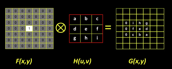
- When convolving a filter with an impulse image, we get the filter back as a result. Similarly if we convolve an image with an impulse we get the original image
Shift invariant
- Operator behaves the same everywhere, i.e. the value of the output depends on the pattern in the image neighborhood, not the position of the neighborhood
Properties of Convolution
- Linear & shift invariant
- Commutative f * g = g * f
- Associative (f * g) * h = g * (f * h)
- Identity unit impulse e = [...,0,0,1,0,0,...]. f * e = f
- Differentiation $$\frac { { \partial }}{ \partial { x } } (f*g)=\frac { { \partial f }}{ \partial { x } }*g $$
Separability
- In some cases, filter is separable, meaning you can get the square kernel H by convolving a single column vector by some row vector
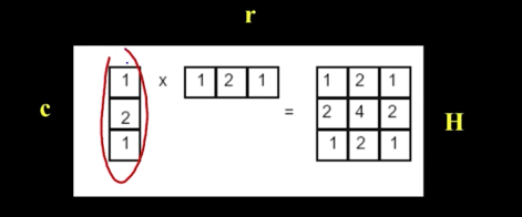
So, now we can do something amazing
G = H * F = (C * R) * F = C * (R * F)
We do two convolutions but each is WNN. So this is useful if W is big enough such that
2WN^2 << W^2*N^2
Boundry Issues
See above example, with mode
Practice Linear Filter
face = messi[60:140, 180:290]
ball = messi[280:340, 330:390]
imshow(face)
imshow(ball)


# no change
f1 = np.array([[0,0,0],[0,1,0],[0,0,0]])
filtered = convolve(green(face), f1, mode='constant')
imshow(filtered)

# Shifted, Notice the very black line at the begining and the end of the
# the last two images for convolution and correlation respectively
f2 = np.array([[0,0,0],[0,0,1],[0,0,0]])
conv = convolve(green(face), f2, mode='constant')
corr = correlate(green(face), f2, mode='constant')
imshow(green(face))
imshow(conv)
imshow(corr)


# Blur (with a box filter)
f3 = 1.0/9.0*np.ones((3,3))
conv = convolve(green(face), f3, mode='constant')
corr = correlate(green(face), f3, mode='constant')
imshow(green(face))
imshow(conv)
imshow(corr)

# twise the impulse - blur >>> Sharpening filter
# Accentuates difference with local average
f4 = np.array([[0,0,0],[0,2,0],[0,0,0]]) - 1.0/9.0*np.ones((3,3))
conv = convolve(green(ball), f4, mode='constant')
corr = correlate(green(ball), f4, mode='constant')
imshow(green(ball))
imshow(conv)
imshow(corr)


# Messi's image is not working well with this filter
f4 = np.array([[0,0,0],[0,1.0,0],[0,0,0]]) - 1.0/9.0*np.ones((3,3))
imshow(green(messi))
for i in range(20):
f4 += np.array([[0,0,0],[0,0.1,0],[0,0,0]])
conv = convolve(green(messi), f4, mode='constant')
#imsave(conv,"%d.jpg" % i)
imshow(conv)


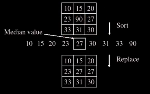
Median Filter
from scipy.ndimage import median_filter
imshow(green(messi))
imshow(salty)
imshow(median_filter(salty,(3,3)))

The following code are not part of this chapter but meant for a friend who asked me for a workflow to extract items and prices from a brochure
# items = cv.imread("items.jpg")
# items = cv.cvtColor(items, cv.COLOR_BGR2RGB)
#imshow(items)
# items = cv.imread("items.jpg")
# items = cv.cvtColor(items, cv.COLOR_BGR2RGB)
# def angle_cos(p0, p1, p2):
# d1, d2 = (p0-p1).astype('float'), (p2-p1).astype('float')
# return abs( np.dot(d1, d2) / np.sqrt( np.dot(d1, d1)*np.dot(d2, d2) ) )
# def find_squares(img):
# img = cv.GaussianBlur(img, (5, 5), 0)
# squares = []
# for gray in cv.split(img):
# for thrs in xrange(0, 255, 150):
# if thrs == 0:
# bin = cv.Canny(gray, 0, 50, apertureSize=5)
# bin = cv.dilate(bin, None)
# else:
# _retval, bin = cv.threshold(gray, thrs, 255, cv.THRESH_BINARY)
# x = cv.findContours(bin, cv.RETR_LIST, cv.CHAIN_APPROX_SIMPLE)
# bin, contours = x[1],x[0]
# for cnt in contours:
# cnt_len = cv.arcLength(cnt, True)
# cnt = cv.approxPolyDP(cnt, 0.02*cnt_len, True)
# if len(cnt) == 4 and cv.contourArea(cnt) > 1000 and cv.isContourConvex(cnt):
# cnt = cnt.reshape(-1, 2)
# max_cos = np.max([angle_cos( cnt[i], cnt[(i+1) % 4], cnt[(i+2) % 4] ) for i in xrange(4)])
# if max_cos < 0.1:
# squares.append(cnt)
# return squares
# gray_image = cv.convertScaleAbs(items)
# squares = find_squares(gray_image)
# cv.drawContours( items, squares, -1, (0, 255, 0), 3 )
# imshow(items)
# s = squares[11]
# def height(s):
# return max(s[3][0],s[2][0]) - min(s[0][0],s[1][0])
# def width(s):
# return max(s[1][1],s[2][1]) - min(s[0][1],s[3][1])
# for s in squares:
# if width(s)< 200 and height(s) < 500:
# try:
# imshow(items[min(s[0][1],s[3][1]):max(s[1][1],s[2][1]),min(s[0][0],s[1][0]):max(s[3][0],s[2][0])])
# except ValueError:
# continue
1D (nx) correlation
%matplotlib inline
def normalize(s):
start = -0.5
end = 0.5
width = end - start
res = (s - s.min())/(s.max() - s.min()) * width + start
return res
signal = (green(messi)[100,:]).astype(np.float64)
signal = normalize(signal)
signal = signal[120:200]
plt.plot(signal)

f = signal[20:30]
plt.plot(f)

norm_c_c = correlate(signal,f)
plt.plot(norm_c_c)

**Note**: The plot is at its maximum from where the snapped were taken from. So, the highest value when these things match. This is the case because the sign matches most at the filter signal. In other words the filter and the signal will have the same signs and thus the multiplication will be at its highest.
Lets do the same with 2D image
imshow(messi)
imshow(face)
########################################################################################
# Author: Ujash Joshi, University of Toronto, 2017 #
# Based on Octave implementation by: Benjamin Eltzner, 2014 <b.eltzner@gmx.de> #
# Octave/Matlab normxcorr2 implementation in python 3.5 #
# Details: #
# Normalized cross-correlation. Similiar results upto 3 significant digits. #
# https://github.com/Sabrewarrior/normxcorr2-python/master/norxcorr2.py #
# http://lordsabre.blogspot.ca/2017/09/matlab-normxcorr2-implemented-in-python.html #
########################################################################################
import numpy as np
from scipy.signal import fftconvolve
def normxcorr2(template, image, mode="full"):
"""
Input arrays should be floating point numbers.
:param template: N-D array, of template or filter you are using for cross-correlation.
Must be less or equal dimensions to image.
Length of each dimension must be less than length of image.
:param image: N-D array
:param mode: Options, "full", "valid", "same"
full (Default): The output of fftconvolve is the full discrete linear convolution of the inputs.
Output size will be image size + 1/2 template size in each dimension.
valid: The output consists only of those elements that do not rely on the zero-padding.
same: The output is the same size as image, centered with respect to the ‘full’ output.
:return: N-D array of same dimensions as image. Size depends on mode parameter.
"""
# If this happens, it is probably a mistake
if np.ndim(template) > np.ndim(image) or \
len([i for i in range(np.ndim(template)) if template.shape[i] > image.shape[i]]) > 0:
print("normxcorr2: TEMPLATE larger than IMG. Arguments may be swapped.")
template = template - np.mean(template)
image = image - np.mean(image)
a1 = np.ones(template.shape)
# Faster to flip up down and left right then use fftconvolve instead of scipy's correlate
ar = np.flipud(np.fliplr(template))
out = fftconvolve(image, ar.conj(), mode=mode)
image = fftconvolve(np.square(image), a1, mode=mode) - \
np.square(fftconvolve(image, a1, mode=mode)) / (np.prod(template.shape))
# Remove small machine precision errors after subtraction
image[np.where(image < 0)] = 0
template = np.sum(np.square(template))
out = out / np.sqrt(image * template)
# Remove any divisions by 0 or very close to 0
out[np.where(np.logical_not(np.isfinite(out)))] = 0
return out
messi_n = green(messi)
face_n = green(face)
# the below command take some time
norm_c_c = normxcorr2(face_n,messi_n)
norm_c_c
def plot_3d(arr):
fig = plt.figure()
ax = fig.gca(projection='3d')
w, h = arr.shape
Y = np.arange(1, w+1)
X = np.arange(1, h+1)
X, Y = np.meshgrid(X, Y)
Z = arr
surf = ax.plot_surface(X, Y, Z, rstride=1, cstride=1, cmap='hot', linewidth=0, antialiased=False)
plot_3d(norm_c_c)

imshow(messi)
imshow(messi2)
Now lets see if we can find Messi's face in the second image using his face in the first image
messi3 = cv.imread("messi5.jpg")
messi3 = cv.cvtColor(messi3, cv.COLOR_BGR2RGB)
messi4 = cv.imread("messi4.jpg")
messi4 = cv.cvtColor(messi4, cv.COLOR_BGR2RGB)
messi3 = resize(messi3,(messi4.shape[1],messi4.shape[0]))
imshow(messi3)
imshow(messi4)
img = green(messi3)
template = green(messi4)
#only the face
template = template[80:200,205:320]
imshow(template)
corr = normxcorr2(template,img,"full")


from numpy import unravel_index
def largest_indices(ary, n):
"""Returns the n largest indices from a numpy array."""
flat = ary.flatten()
indices = np.argpartition(flat, -n)[-n:]
indices = indices[np.argsort(-flat[indices])]
return np.unravel_index(indices, ary.shape)
x,y = unravel_index(corr.argmax(), corr.shape)
w,h = template.shape
im = messi3.copy()
im[:,:,0] = img
im[:,:,1] = img
im[:,:,2] = img
im[x-w:x,y-h:y] = messi3[x-w:x,y-h:y]
print ("******Template******")
imshow(template)
print ("******Match******")
imshow(im)

grayImg = 255-255*(corr + corr.max())/(corr.max()-corr.min())
grayImg = grayImg.astype(np.uint8)
imshow(grayImg)

fig = plt.gcf()
fig.set_size_inches(18.5, 10.5)
x = np.ones((50,50))*255
x[:,10:20] = 0
ax = plt.subplot(131)
ax.imshow(x)
# Plotting scanline
ax = plt.subplot(132)
ax.plot(x[10,:])
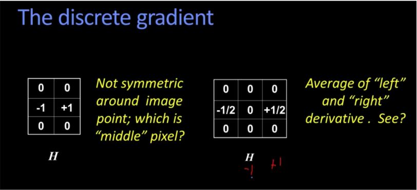
### Finding Derivative
### https://plot.ly/python/numerical-differentiation/
x10 = np.arange(50)
y = x[10,:]
dy = np.zeros(y.shape,np.float)
dy[0:-1] = np.diff(y)/np.diff(x10)
dy[-1] = (y[-1] - y[-2])/(x10[-1] - x10[-2])
ax = plt.subplot(133)
ax.plot(dy)


zebra = cv.imread("zebra.jpg")
Gradient Simple Implementation
def grad_x(img):
img2 = img.astype(np.float)
dimg = np.zeros(img.shape).astype(np.float)
for i in range(img2.shape[0]):
y = img2[i,:]
x = np.arange(img2.shape[1]).astype(np.float)
dy = np.zeros(y.shape,np.float).astype(np.float)
dy[0:-1] = np.diff(y)/np.diff(x)
dy[-1] = (y[-1] - y[-2])/(x[-1] - x[-2])
dimg[i] = dy
return dimg
def grad_y(img):
img2 = img.astype(np.float)
dimg = np.zeros(img.shape).astype(np.float)
for i in range(img2.shape[1]):
y = img2[:,i]
x = np.arange(img2.shape[0]).astype(np.float)
dy = np.zeros(y.shape,np.float).astype(np.float)
dy[0:-1] = np.diff(y)/np.diff(x)
dy[-1] = (y[-1] - y[-2])/(x[-1] - x[-2])
dimg[:,i] = dy
return dimg
def display_grid(imgs,titles):
plt.gray()
plt.figure(figsize=(20,20))
plt.subplot(221)
plt.imshow(imgs[0])
plt.title(titles[0], size=20)
if len(imgs)> 1:
plt.subplot(222)
plt.imshow(imgs[1])
plt.title(titles[1], size=20)
if len(imgs)> 2:
plt.subplot(223)
plt.imshow(imgs[2])
plt.title(titles[2], size=20)
if len(imgs)> 3:
plt.subplot(224)
plt.imshow(imgs[3])
plt.title(titles[3], size=20)
plt.show()
def display_pair(imgs,titles):
plt.gray()
plt.figure(figsize=(20,20))
plt.subplot(121)
ax = plt.gca()
ax.xaxis.set_major_locator(plt.NullLocator())
ax.yaxis.set_major_locator(plt.NullLocator())
plt.imshow(imgs[0])
plt.title(titles[0], size=20)
if len(imgs)> 1:
plt.subplot(122)
plt.imshow(imgs[1])
plt.title(titles[1], size=20)
ax = plt.gca()
ax.xaxis.set_major_locator(plt.NullLocator())
ax.yaxis.set_major_locator(plt.NullLocator())
plt.show()
### Smoothing first
s = 1
zebra_res = resize(green(zebra),(130,200))
kernel = np.ones((s,s),np.float32)/s**2
dst = cv.filter2D(zebra_res,-1,kernel)
### Taking the gradient
xdimg = grad_x(dst).astype(np.uint8)
ydimg = grad_y(dst).astype(np.uint8)
display_grid([dst,xdimg,ydimg],["original","diff_x","diff_y"])

Using sobel operator (skimage library)
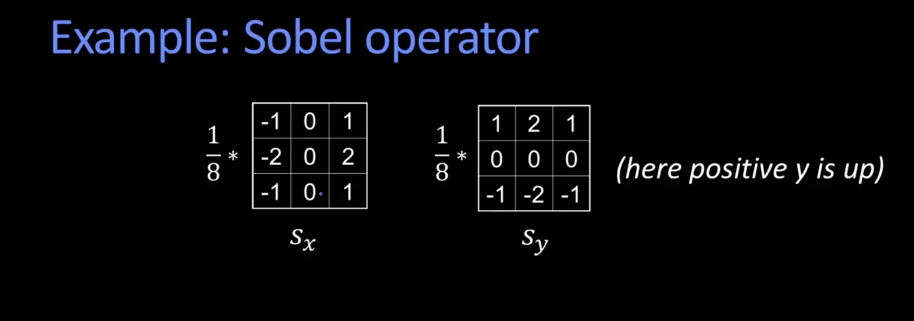
%matplotlib inline
from skimage import filters
def sobel(img):
edges_x = filters.sobel_h(img)
edges_y = filters.sobel_v(img)
edges = filters.sobel(img)
return edges_x,edges_y,edges
def prewitt(img):
edges_x = filters.prewitt_h(img)
edges_y = filters.prewitt_v(img)
edges = filters.prewitt(img)
return edges_x,edges_y,edges
def roberts(img):
edges_x = filters.roberts_pos_diag(img)
edges_y = filters.roberts_neg_diag(img)
edges = filters.roberts(img)
return edges_x,edges_y,edges
x1,y1,d1 = sobel(zebra_res)
#display_grid([zebra_res,x,y,d],["original","sobel_x","sobel_y","sobel"])
x2,y2,d2 = prewitt(zebra_res)
#display_grid([zebra_res,x,y,d],["original","prewitt_x","prewitt_y","prewitt"])
x3,y3,d3 = roberts(zebra_res)
#display_grid([zebra_res,x,y,d],["original","roberts_pose_diag","roberts_neg_diag","roberts"])
display_grid([zebra_res,d1,d2,d3],["original","sobel","prewitt","roberts"])

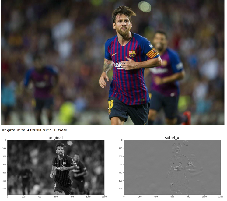
Lets try with Messi
x,y,d = sobel(green(messi))
display_grid([green(messi),x,y,d],["original","sobel_x","sobel_y","sobel"])

🤩 Lovely 🤩
**Visit the implementation for the previous filters function in the library skimage
Canny Edge Operator
- Filter image with derivative of Gaussian
- Find Magnitude and orientation of gradient
- Non-maximum suppression: Thin mult-pixel wide "ridges" down to single pixel width
- Linking and thresholding (hysteresis):
- Define two thresholds: low and high
- Use the high threshold to start edge curves and the low threshold to continue them
edges = cv.Canny(green(messi),100,200)
edges1 = cv.Canny(green(messi),100,100)
edges2 = cv.Canny(green(messi),50,50)
display_grid([green(messi),edges,edges1,edges2],["Original","100X200","100X100","50X50"])

Laplacian

edges = cv.Laplacian(green(messi),cv.CV_64F)
edges1 = cv.Laplacian(green(messi),cv.CV_64F,ksize=7)
edges2 = cv.Laplacian(green(messi),cv.CV_64F,ksize=11)
display_grid([green(messi),edges,edges1,edges2],["Original","Laplacian","Laplacian 5","Laplacian 11"])

Parametric model
- A parametric model can represent a class of instances where each is defined by a value of the parameters
- Examples include lines, or circles, or even a parameterized template
Fitting a parametric model
- Choose a parametric model to represent a set of features
- Membership criterion is not local
- can't tell whether a point in the image belongs to a given model just by looking at that point
- Computational complexity is important
- not feasible to examine possible parameter setting
Example: Line fitting
building = imread("building.png")
road = imread("road.png")
imshow(building)
imshow(road)


building = imread("building2.jpg")
building = resize(building,(520,350))
imshow(building)

Difficulty of line fitting
- Extra edge points (clutter), multiple models
- Only some parts of each line detected, and some parts are missing
- Noise in measured edge points, orientation
edges = cv.Canny(green(building),100,100)
imshow(edges)

Voting
voting is a general technique where we let the features vote for all models that are compatible with it.
- Cycle through features, each casting votes for model parameters
- Look for model parameters that receive a lot of votes
Why it works?!!
- Noise & clutter features will cast votes too, but typically their votes should be inconsistent with the majority of "good" features.
- Ok if some features not observed, as model can span multiple fragments
Fitting lines
To fit lines we need to answer few questions:
- Given points that belongs to a line, what is the line?
- How many lines are there?
- Which points belong to which lines?
Hough Transform
It is a voting technique that can be used to answer all of these. Its main idea is:
1. Each edge point votes for compatible lines.
2. Look for lines that get many votes
Hough Space

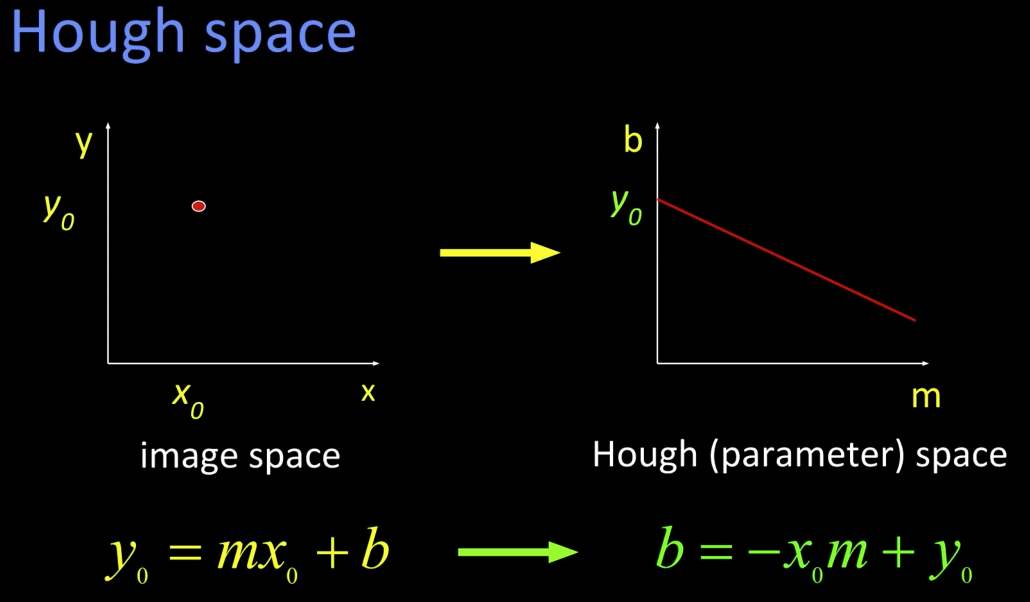
The line has to point where the two lines intersect at hough space.
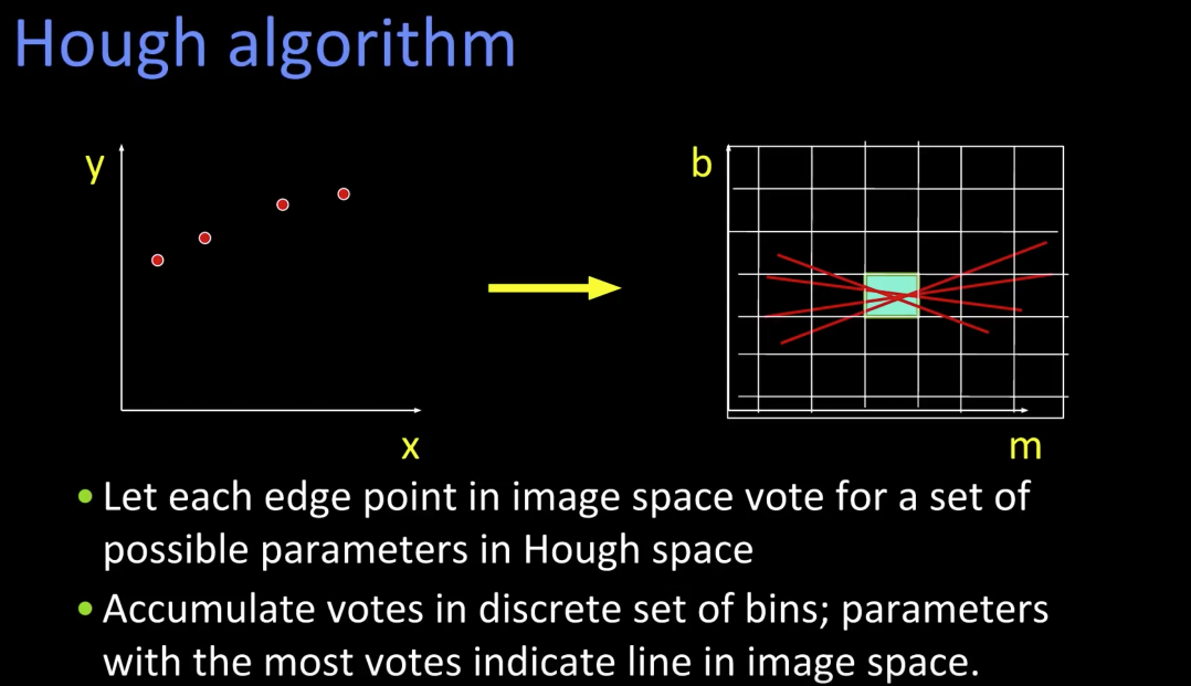

Hough transform algorithm
Using the polar parameterization:
$$ x*cos(\theta) - y*sin(\theta) = d $$
And a Hough Accumulator Array(keeps the votes)

- Initialize H[d, $\theta$] = 0
- For each edge point in E(x,y) in the image
- for $\theta$ = 0 to 180
- d = $x*cos(\theta) - y*sin(\theta)$
- H[d,$\theta$] += 1
- for $\theta$ = 0 to 180
- Find the value(s) of (d,$\theta$) where H[d,$\theta$] is maximum
- The detected line in the image is given by $$ d = x*cos(\theta) - y*sin(\theta) $$
https://docs.opencv.org/2.4/doc/tutorials/imgproc/imgtrans/hough_lines/hough_lines.html
def find_lines(img,minLineLength=100,maxLineGap=20,rho = 1,canny_t=(150,150),top=10):
img2 = img.copy()
gimg2 = gray(img)
edges = cv.Canny(gimg2,canny_t[0],canny_t[1],apertureSize =3)
imshow(edges)
lines = cv.HoughLinesP(edges,
rho = rho,
theta = np.pi/180,threshold = 1,
minLineLength = minLineLength,
maxLineGap = maxLineGap)
try:
mag = [np.sqrt(np.power(y2-y1,2)+np.power(x2-x1,2)) for x1,y1,x2,y2 in lines[0]]
mag = zip(np.arange(len(mag)),mag)
mag = sorted(mag, key=lambda tup: tup[1],reverse=True)
lines = lines[0]
for i in range(min(len(mag),top)):
index = mag[i][0]
x1,y1,x2,y2 = lines[index]
cv.line(img2,(x1,y1),(x2,y2),(0,255,0),2)
except:
raise
imshow(img2)
find_lines(building)


Now lets try Messi
find_lines(messi,minLineLength=100,maxLineGap=20,rho=1,canny_t=(200,100),top=10)


🤨 Really!!! 🤨
Hough Transform for Circles
Circle: center (a,b) and radius r $$({x}_{i} - a)^2 + ({y}_{i} - b)^2 = r^2$$
For a fixed radius r, uknown gradient direction:
- Votes for circle
%matplotlib inline
circle1 = plt.Circle((.5, .5), 0.2, color=None,fill=False)
fig, ax = plt.subplots(1,2)
fig.set_size_inches(10,6)
ax1,ax2 = ax[0],ax[1]
ax1.add_artist(circle1)
ax1.plot([0.58],[0.68],'o')
ax1.plot([0.60],[0.332],'o')
ax1.plot([0.3],[0.5],'o')
ax1.set_xlim(0,1)
ax1.set_ylim(0,1)
ax1.set_ylabel("y")
ax1.set_xlabel("x")
ax1.set_title("Image space")
ax1.set_yticks([])
ax1.set_xticks([])
circle2 = plt.Circle((.3, .5), 0.2, color=None,fill=False)
ax2.plot([0.3],[0.5],'o',color='g')
circle3 = plt.Circle((.60, .332), 0.2, color=None,fill=False)
ax2.plot([0.6],[0.332],'o',color='orange')
circle4 = plt.Circle((.58, .68), 0.2, color=None,fill=False)
ax2.plot([0.58],[0.68],'o',color='b')
ax2.plot([0.5],[0.5],'o',color='r')
ax2.add_artist(circle2)
ax2.add_artist(circle3)
ax2.add_artist(circle4)
ax2.annotate("", xy=(.12, .4), xytext=(.3, .5),arrowprops=dict(label="",arrowstyle="->",color="blue"))
ax2.annotate("r", xy=(.22, .42))
ax2.annotate("", xy=(.5, .5), xytext=(0.8, 0.8),arrowprops=dict(label="",arrowstyle="->",color="purple"))
ax2.annotate("Most votes\n for center\n occur here",xy=(0.7, 0.8),)
ax2.set_xlim(0,1)
ax2.set_ylim(0,1)
ax2.set_ylabel("b")
ax2.set_xlabel("a")
ax2.set_title("Hough space")
ax2.set_yticks([])
ax2.set_xticks([])
plt.show()

- For uknown radius r, no gradient:
- each points for a cone
%matplotlib inline
from matplotlib.patches import Circle, PathPatch
# register Axes3D class with matplotlib by importing Axes3D
from mpl_toolkits.mplot3d import Axes3D
import mpl_toolkits.mplot3d.art3d as art3d
from matplotlib.text import TextPath
from matplotlib.transforms import Affine2D
fig = plt.figure()
ax = fig.add_subplot(111, projection='3d')
# Draw a circle on the x=0 'wall'
ps = []
for i in range(1,10):
p = Circle((10, 10), i,fill=False)
ax.add_patch(p)
art3d.pathpatch_2d_to_3d(p, z=i, zdir="z")
ax.set_xlabel("a")
ax.set_ylabel("b")
ax.set_zlabel("r")
ax.set_xlim(0, 20)
ax.set_ylim(0, 20)
ax.set_zlim(0, 20)
ax.set_xticks([])
ax.set_yticks([])
ax.set_zticks([])
plt.show()

Algorithm
- For e in edges(x,y)
- For r in all(radii):
- For $\theta$ in all(gradient directions):
- a = x - r*cos($\theta$)
- b = y + r*sin($\theta$)
- H[a,b,r] += 1
- For $\theta$ in all(gradient directions):
- For r in all(radii):
def find_circles(img,minDist=100,accValue=200):
output = img.copy()
grayim = gray(output)
circles = cv.HoughCircles(grayim, cv.HOUGH_GRADIENT, accValue, minDist)
# ensure at least some circles were found
if circles is not None:
# convert the (x, y) coordinates and radius of the circles to integers
circles = np.round(circles[0, :]).astype("int")
# loop over the (x, y) coordinates and radius of the circles
for (x, y, r) in circles:
# draw the circle in the output image, then draw a rectangle
# corresponding to the center of the circle
cv.circle(output, (x, y), r, (0, 255, 0), 4)
cv.rectangle(output, (x - 5, y - 5), (x + 5, y + 5), (0, 128, 255), -1)
# show the output image
imshow(np.hstack([output]))
soda = imread("detect_circles_soda.jpg")
find_circles(soda)
circles = imread("circles.jpg")
find_circles(circles,10,15)


Now lets try Messi
find_circles(messi,5,40)

🤔 MMM. Not very impressive!!! 🤔
- Non-analytic models
- Parameters express variation in pose or scale of fixed but arbitrary shape (that was then)
- Visual code-word based feature
- Not edges but detected templates learned from models (this is "now")
Training: build a Hough table
- At each boundry point, compute displacement vector: r = c - ${p}_{i}$
- Measure the gradient angle $\theta$ at the bounary point
- Store the displacement in a table indexed by $\theta$

Recognition
- At each boundry point, measure the gradient angle $\theta$
- Look up all displacements in $\theta$ displacement table.
- Vote for a center at each displacement.

Algorithm
If orientation is known:
- For each edge point:
- Compute gradient direction $\theta$
- Retrieve displacement vector r to vote for reference point.
- Peak in this Hough space (X,Y) is reference point with most supporting edges
If orientation is unknown:
- for each edge point
- For each possible master $\theta$*
- Compute gradient direction $\theta$
- New $\theta$' = $\theta - \theta$*
- For $\theta$' retrieve displacement vectors to vote for reference point.
- For each possible master $\theta$*
- Peak in this Hough space (now, X,Y,$\theta$*) is reference point with most supporting edges
If scale S is unknonw:
- for each edge point
- For each possible master $\theta$*
- Compute gradient direction $\theta$
- For $\theta$' retrieve displacement vectors r.
- Vote r scaled by S for reference point.
- For each possible master $\theta$*
- Peak in this Hough space (now, X,Y,S) is reference point with most supporting edges
Application in Recognition
- Instead of indexing displacements by gradient orientation, index by "visual codeword"
display_pair([imread("car.png"),imread("car_wheel.png")],
["Training image",
"Visual Codeword with displacement vectors"])

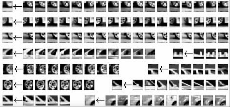
- Take an image operator
- Pull out all the interesting points on a bunch of training images
- You collect the little image patch right around those points
- You cluster them
- The center of the clusters are referred to as visual codewords
Training: Displacements
3) For each codebook entry, store all displacements relative to object center

Run-Time

To identify the car, and suppose we have only one feature (e.g. tire), than we find the place of the tires using the training codewords, and then use the displacement vectors associated with the best matched codewords to identify the point where most vectors point to.
Now lets bring magisterial Messi back (He scored 2 goals against Alave's two days ago in the first La-liga match 2018)
## Sift is no longer an opensource, unless you combile opencv_contrib from the source
# def gen_sift_features(gray_img):
# sift = cv.xfeatures2d.SIFT_create()
# kp, desc = sift.detectAndCompute(gray_img, None)
# return kp, desc
# def show_sift_features(gray_img, color_img, kp):
# fig, ax = plt.subplots()
# fig.set_size_inches(20,20)
# return ax.imshow(cv.drawKeypoints(gray_img, kp, color_img.copy()))
# messi_alaves = imread("messi_alaves.jpg")
# imshow(messi_alaves)
# # generate SIFT keypoints and descriptors
# messi_kp, messi_desc = gen_sift_features(gray(messi_alaves))
# x,y,d = sobel(green(messi_alaves))
# display_grid([green(messi_alaves),x,y,d],["original","sobel_x","sobel_y","sobel"])
# print ('Here are what SIFT features look like for Messi vs Alaves image:')
# show_sift_features(gray(messi_alaves), messi_alaves, messi_kp);
Sift is no longer an opensource, unless you compile opencv_contrib from the source. However, below is an image of the ouput of the previous code
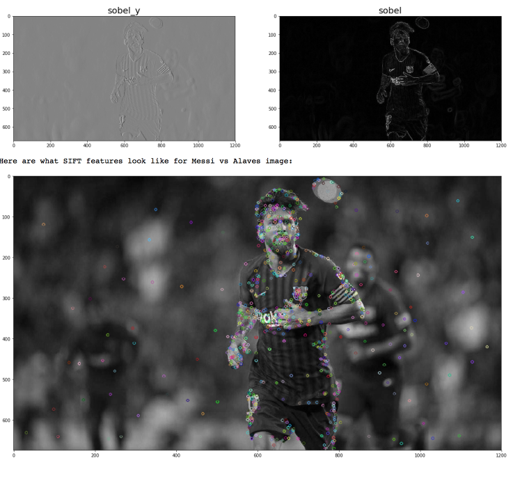
Full Example: http://ianlondon.github.io/blog/how-to-sift-opencv/
Decomposing an image: Basis sets
A basis set is (edit from Wikipedia):
A basis B of a vector space V is a linearly independent subset of V that spans V
Suppose that B = {v1,...,vn} is a finite subset of a vector space V over a field F (such as the real or complex numbers R or C). Then B is a basis if it satisfies the following conditions:- Linear independence:
For all ${a}_{1}$,...,${a}_{n} \in$ F, if ${a}_{1}{v}_{1}$ + ...+ ${a}_{n}{v}_{n}$ = 0, then necessarily
${a}_{1} = ...= {a}_{n} = 0$ - Spanning property,
- For every $x$ in V it is possible to choose ${a}_{1}$,...,${a}_{n} \in F$ such that ${x} = {a}_{1}{v}_{1} + ... + {a}_{n}{v}_{n} = 0$
- Linear independence:
Images as points in a vector space
Consider an image as a point in a NxN size space - can rasterize into a single vector
$[{x}_{00},{x}_{10},{x}_{20},{x}_{(n-1)0},{x}_{01},...,{x}_{(n-1)(n-1)}]^T$
- The "Normal" basis is just the vectors:
$[0 0 0 0 ... 0 1 0 0 0 0 0 0 0 ... 0]^T$
- Independent
- Can create any image
- Not very helpful
A nice set of basis
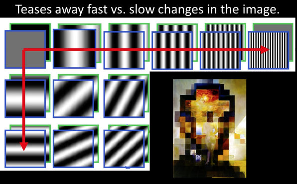
x = np.linspace(np.pi, 2*np.pi, 201)
fig, ax = plt.subplots(7,1)
fig.set_size_inches(7,20)
fs = [
lambda i: 1,
lambda i: np.sin(3*i),
lambda i: 0.5*np.sin(10*i+np.pi),
lambda i: 0.3*np.sin(15*i),
lambda i: 0.2*np.sin(30*i+np.pi)
]
ax[0].plot([0]*75+[1]*75+[0]*75)
ax[0].set_title("Target")
c = 1
for f in fs:
ax[c].plot([f(xi) for xi in x])
ax[c].set_title("f%d" % c)
c+= 1
ax[6].plot([sum([f(xi) for f in fs[:-1]]) for xi in x])
ax[6].set_title("f%d + f%d + f%d" % (0,1,2))

Frequency Spectra- Series
at = lambda f,t: np.sin(2*np.pi*f*t)
bt = lambda f,t: 0.333*np.sin(2*np.pi*3*f*t)
gt = lambda f,t: at(f,t) + bt(f,t)
x = np.linspace(np.pi, 2*np.pi, 201)
fig, ax = plt.subplots(2,2)
fig.set_size_inches(8,7)
ax[0,0].plot([at(2,xi) for xi in x])
ax[0,1].plot([bt(2,xi) for xi in x])
ax[1,0].plot([gt(2,xi) for xi in x])
ax[1,1].bar([0,1,2],[1,0,0.3])
ax[1,1].set_title("One form of spuctrum")

at = lambda t,k: + (1.0/k)*np.sin(2*np.pi*k*t)
Ampl = 1
x = np.linspace(np.pi, 2*np.pi, 201)
fig, ax = plt.subplots(2,2)
fig.set_size_inches(15,7)
pis = [(0,0),(0,1),(1,0),(1,1)]
for i in range(1,5):
y = np.array([at(xi,1) for xi in x])
for k in range(1,i):
y += Ampl*np.array([at(xi,2*k+1) for xi in x])
ax[pis[i-1][0],pis[i-1][1]].plot(y)

plt.bar(np.arange(10),[0.7**x for x in np.arange(10)])
ax = plt.gca()
ax.xaxis.set_major_locator(plt.NullLocator())
ax.yaxis.set_major_locator(plt.NullLocator())
ax.set_xlabel("frequency")

Fourier Transform
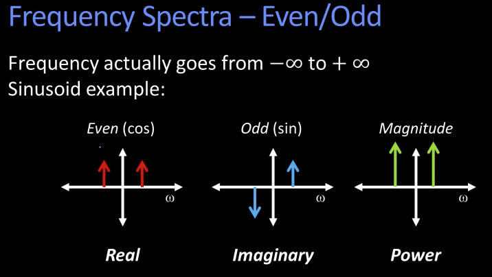
We want to understand the frequency $\omega$ of our signal. So, lets reparametrize the signal by $\omega$ insead of x:
f(x) ----> [Fourier Transform] -----> F($\omega$)
Asin($\omega$x + $\phi$)
For every $\omega$ from 0 to $\infty$ (actually -$\infty$ to $\infty$), F($\omega$) holds the amplitude A and phase f of the corresponding sinusoid
How can F hold both amplitude and phase?
Complex number trick!
Computing FT: Just a basis
The infinite integral of the product of two sinusoids of different frequency is zero. (Why?)
f1 = lambda i: np.sin(3*i)
f2 = lambda i: np.sin(4*i)
x = np.linspace(np.pi, 2*np.pi, 201)
plt.plot([f1(xi) for xi in x])
plt.plot([f2(xi) for xi in x])

And if same frequency the integral is infinite:
... if $\phi$ and $\varphi$ not exactly $\frac{\pi}{2}$ out of phase (sin anc cos)
So, suppose f(x) is a cosine wave of freq $\omega$:
Then: $$C(u) = \int_{-\infty}^\infty f(x)cos(2\pi u x) dx$$
which is infinite if u is equal to $\omega$ or $-\omega$ and zero otherwise
omega = 10
x = 10
f = lambda i: np.cos(2*np.pi*omega*x)
x = np.linspace(np.pi, 2*np.pi, 201)
plt.plot([f1(xi) for xi in x])
ax = plt.gca()

- We can do that for all frequecncies u
- But we'd have to do that for all phases, don't we???
- No! Any phase can be created by a weighted sum of cosine and sine. Onle need each piece
$$C(u) = \int_{-\infty}^\infty f(x)cos(2\pi u x) dx$$ $$S(u) = \int_{-\infty}^\infty f(x)sin(2\pi u x) dx$$
omega = 1
f1 = lambda i: np.cos(2*np.pi*omega*i)
f2 = lambda i: np.sin(2*np.pi*omega*i)
x = np.linspace(np.pi, 2*np.pi, 100)
plt.plot([f1(xi) for xi in x])
plt.plot([f2(xi) for xi in x])
ax = plt.gca()

Fourier Transform - more formally
Represent the signal as an infinite weighted sum of an infinite number of sinusoids:
$$C(u) = \int_{-\infty}^\infty f(x)e^{-i2\pi u x} dx$$
Spatial Domain(x) ---> Frequency Domain ($\omega$ or u or even s) Frequency Spectrum F(u) or F($\omega$)
Inverse Fourier Transform (IFT)
$$f(x) = \int_{-\infty}^\infty F(u)e^{i2\pi u x} du$$

Fourier Transform - limitations
- The integral $\int_{-\infty}^\infty f(x)e^{-i2\pi u x} dx$ exists if the function f is integrable:
$$\int_{-\infty}^\infty | f(x) | dx < \infty$$ - If there is a bound of width T outside of which f is zero than obviosly could integrate from just $-\frac{T}{2}$ to $\frac{T}{2}$
The Discrete Fourier Transform
$$F(k) = \frac{1}{N} \sum_{x=0}^{x=N-1}f(x)e^\frac{-i2\pi k x}{N} $$
... where x is discrete and goes from the start of the signal to the end (N-1) ... and k is the number "cycles per period of the signal" or "cycles per image.
Only makes sense k = $\frac{N}{2}$ to $\frac{N}{2}$ why? What's highest frequency you can unambiguously have in a discrete image?
2D Fourier Transforms
- The two dimensional version:.
$$F(u,v) = \int_{-\infty}^\infty \int_{-\infty}^\infty f(x,y)e^{-i2\pi ux + vy} dx dy$$
And the 2D Discrete FT: $$F(k_x,k_y) = \frac{1}{N} \sum_{x=0}^{x=N-1}\sum_{y=0}^{y=N-1} f(x)e^\frac{-i2\pi(k_x x + k_y y)}{N} $$
Works best when you put the origin of k in the middle
Examples
%matplotlib inline
def normalize_img(s):
start = 0
end = 255
width = end - start
res = (s - s.min())/(s.max() - s.min()) * width + start
return res
A = .8
f = 5
t = np.arange(0,1,.01)
phi = np.pi/4
x = normalize_img(A*np.cos(2*np.pi*f*t + phi))
sinusoid = np.array([x]*len(t)).astype(np.uint8)
f = np.fft.fft2(sinusoid)
fshift = np.fft.fftshift(f)
magnitude_spectrum = np.abs(fshift)
display_pair([sinusoid,magnitude_spectrum],["Sinusoid","FFT"])

st = sinusoid.transpose()
f = np.fft.fft2(st)
fshift = np.fft.fftshift(f)
magnitude_spectrum = np.abs(fshift)
display_pair([st,magnitude_spectrum],["Sinusoid","FFT"])

Linearity of Sum
A = .8
f = 5
fx=1/20.0
fy=1/20.0
t = np.arange(0,1,.01)
phi = np.pi/4
s = lambda i,j : A*np.cos(2*np.pi*f*(fx*i+fy*j))
sinusoid1 = normalize_img(np.array([[s(i,j) for i in x] for j in y])).astype(np.uint8)
ft = np.fft.fft2(sinusoid1)
fshift = np.fft.fftshift(ft)
ms1 = np.abs(fshift)
f = 20
f = 5
fx=1/10.0
fy=0
s = lambda i,j : A*np.sin(2*np.pi*f*(fx*i+fy*j))
sinusoid2 = normalize_img(np.array([[s(i,j) for i in x] for j in y])).astype(np.uint8)
ft = np.fft.fft2(sinusoid2)
fshift = np.fft.fftshift(ft)
ms2 = np.abs(fshift)
display_pair([sinusoid1,ms1],["Sinusoid","FFT"])
display_pair([sinusoid2,ms2],["Sinusoid","FFT"])
display_pair([sinusoid1+sinusoid2,ms1+ms2],["Sinusoid","FFT"])


Now lets bring magisterial Messi back (Tomorrow playing against Valladolid)
ft = np.fft.fft2(gray(messi))
fshift = np.fft.fftshift(ft)
ms = 20*np.log(np.abs(fshift))
ms = normalize_img(ms).astype(np.uint8)
display_pair([gray(messi),ms],["Messi","FFT"])

def normalize_img(s):
start = 0
end = 255
width = end - start
res = (s - s.min())/(s.max() - s.min()) * width + start
return res
def fft(img):
ft = np.fft.fft2(img)
fshift = np.fft.fftshift(ft)
ms = 20*np.log(np.abs(fshift))
ms = normalize_img(ms).astype(np.uint8)
return ms
def hpfm(img):
rows, cols = img.shape
crow,ccol = rows//2 , cols//2
ft = np.fft.fft2(gray(messi))
fshift = np.fft.fftshift(ft)
fshift[crow-30:crow+30, ccol-30:ccol+30] = 0
f_ishift = np.fft.ifftshift(fshift)
img_back = np.fft.ifft2(f_ishift)
img_back = np.abs(img_back)
return img_back
display_pair([gray(messi),hpfm(gray(messi))],["Messi","High Pass Filter (Edge)"])

"""
The sine wave is important in physics because it retains
its wave shape when added to another sine wave of the same frequency
and arbitrary phase and magnitude. It is the only periodic waveform
that has this property. This property leads to its importance in Fourier
analysis and makes it acoustically unique.
"""
sin = lambda t,k,A,phi: + A*np.sin(2*np.pi*k*t + phi)
x = np.linspace(np.pi, 2*np.pi, 201)
fig,ax = plt.subplots(2,1)
ax[0].plot([sin(xi,2,1,0) for xi in x])
ax[0].plot([sin(xi,2,1,0) + sin(xi,2,2,1) for xi in x])
ax[1].plot([sin(xi,2,1,0) for xi in x])
ax[1].plot([sin(xi,2,1,0) + sin(xi,1,1,0) for xi in x])

Fourier Transform and Convolution
Let g = f * h
then,
$$G(u) = \int_{-\infty}^\infty g(x)e^{-i2\pi u x} dx$$
$$= \int_{-\infty}^\infty \int_{-\infty}^\infty f(\tau)h(x-\tau)e^{-i2\pi ux} d\tau x$$
$$= \int_{-\infty}^\infty \int_{-\infty}^\infty [f(\tau)e^{-i2\pi ux} d\tau][h(x-\tau)e^{-i2\pi u(x-\tau)} dx]$$
$$= \int_{-\infty}^\infty [f(\tau)e^{-i2\pi ux} d\tau]\int_{-\infty}^\infty[h(x')e^{-i2\pi u(x')} dx']$$ $$= F(u)H(u)$$
| Spatial Domain (x) | Frequency Domain(u) | |
|---|---|---|
| g = f \* h | <----> | G = F $\cdot$ H |
| g = f $\cdot$ h | <----> | G = F \* H |
Example use: Smooting/Blurring
- We want a smoothed function of f(x)
$$g(x) = f(x) * h(x)$$
- We can use a Gaussian kernal
$$h(x) = \frac{1}{\sqrt{2\pi \sigma}}e^{-\frac{x^2}{2\sigma^2}}$$
- The Fourier transform of a Gaussian is a Gaussian
$$H(x) = e^{-\frac{(2\pi u)^2\sigma^2}{2}}$$
- Convolution in space is multiplication in freq: $$G(u) = F(u) \cdot H(u)$$
import scipy.ndimage.filters as filter
from scipy.signal import convolve2d
from IPython.display import HTML
def normalize(s):
start = 0.0
end = 255.0
width = end - start
res = (s - s.min())/(s.max() - s.min()) * width + start
return res.astype(np.uint8)
def display_triple(imgs,titles):
plt.gray()
plt.figure(figsize=(20,20))
plt.subplot(131)
ax = plt.gca()
ax.xaxis.set_major_locator(plt.NullLocator())
ax.yaxis.set_major_locator(plt.NullLocator())
plt.imshow(imgs[0])
plt.title(titles[0], size=20)
if len(imgs)> 1:
plt.subplot(132)
plt.imshow(imgs[1])
plt.title(titles[1], size=20)
if len(imgs)> 2:
plt.subplot(133)
plt.imshow(imgs[2])
plt.title(titles[2], size=20)
ax = plt.gca()
ax.xaxis.set_major_locator(plt.NullLocator())
ax.yaxis.set_major_locator(plt.NullLocator())
plt.show()
rows, cols = gray(messi).shape
n = 15
kernal = np.ones((n,n))
#kernal /= np.sum(kernal)
conv = convolve2d(gray(messi), kernal, mode='same')
display(HTML('<strong><span style="color:green">Using convolution</span></strong><br/>'))
display_pair([gray(messi),conv],["Original","Filtered"])
messi_dft = cv.dft(np.float32(gray(messi)),flags = cv.DFT_COMPLEX_OUTPUT)
messi_dft_shift = np.fft.fftshift(messi_dft)
messi_ms = normalize(20*np.log(cv.magnitude(messi_dft_shift[:,:,0],messi_dft_shift[:,:,1])))
# create a mask first, center square is 1, remaining all zeros
crow,ccol = int(rows/2) , int(cols/2)
mask = np.zeros((rows,cols,2),np.float32)
n = 7
mask[crow-n:crow+n, ccol-n:ccol+n] = 1.0
mask_dft = cv.dft(np.float32(mask),flags = cv.DFT_COMPLEX_OUTPUT)
mask_dft_shift = np.fft.fftshift(mask_dft)
mask_ms = normalize(cv.magnitude(mask_dft_shift[:,:,0],mask_dft_shift[:,:,1]))
display(HTML('<strong><span style="color:green">Using FFT</span></strong><br/>'))
# Multiplying filter with messi_dft
mul = messi_dft_shift*mask_dft_shift
mul_ms = normalize(cv.magnitude(mul[:,:,0],mul[:,:,1]))
display_triple([messi_ms,mask_ms,mul_ms],["|F(u,v)|","|H(Sx,Sy)|", "|G(Sx,Sy)|"])
# reversing image
f_ishift = np.fft.ifftshift(mul)
img_back = cv.idft(f_ishift)
img_back = np.fft.ifftshift(img_back)
img_back = cv.magnitude(img_back[:,:,0],img_back[:,:,1])
display_pair([gray(messi),img_back],["Original","Filtered"])


Low and High Pass filtering
display_pair([gray(messi),messi_ms],["Spatial Domain","Frequency Domain"])
display(HTML('<strong><span style="color:green">Low Passing Filter</span></strong><br/>'))
def createCircularMask(h, w, center=None, radius=None):
if center is None: # use the middle of the image
center = [int(w/2), int(h/2)]
if radius is None: # use the smallest distance between the center and image walls
radius = min(center[0], center[1], w-center[0], h-center[1])
Y, X = np.ogrid[:h, :w]
dist_from_center = np.sqrt((X - center[0])**2 + (Y-center[1])**2)
mask = dist_from_center <= radius
return mask
def reverse_fft(fft_img):
f_ishift = np.fft.ifftshift(fft_img)
img_back = cv.idft(f_ishift)
img_back = cv.magnitude(img_back[:,:,0],img_back[:,:,1])
return img_back
h,w = messi_ms.shape
center = [int(w/2), int(h/2)]
mask = createCircularMask(h, w, center=center,radius=40)
masked_img = messi_dft_shift.copy()
masked_img[~mask] = 0
dis_masked_img = messi_ms.copy()
dis_masked_img[~mask] = 0
display_pair([messi_ms,dis_masked_img],["FFT Domain","Low Pass Filter"])
display(HTML('<strong><span style="color:red">Notice the ringing as in the licture</span></strong><br/>'))
display_triple([gray(messi),dis_masked_img,reverse_fft(masked_img)],
["Original","FFT LPF","Ringed Image"])
display(HTML('<strong><span style="color:green">High Passing Filter</span></strong><br/>'))
masked_img[mask] = 0
masked_img = messi_dft_shift.copy()
masked_img[mask] = 0
dis_masked_img = messi_ms.copy()
dis_masked_img[mask] = 0
display_pair([messi_ms,dis_masked_img],["FFT Domain","High Pass Filter"])
display(HTML('<strong><span style="color:red">High Pass Filter is edge detection</span></strong><br/>'))
display_triple([gray(messi),dis_masked_img,reverse_fft(masked_img)],
["Original","FFT LPF","HPF Image"])


Properties of Fourier Transform
| Spatial Domain (x) | Frequency Domain(u) | ||
|---|---|---|---|
| Linearity | $$c_1f(x) + c_2g(x)$$ | $$c_1F(u) + c_2G(u)$$ | |
| Convolution | $$f(x)g(x)$$ | $$F(u)G(u)$$ | |
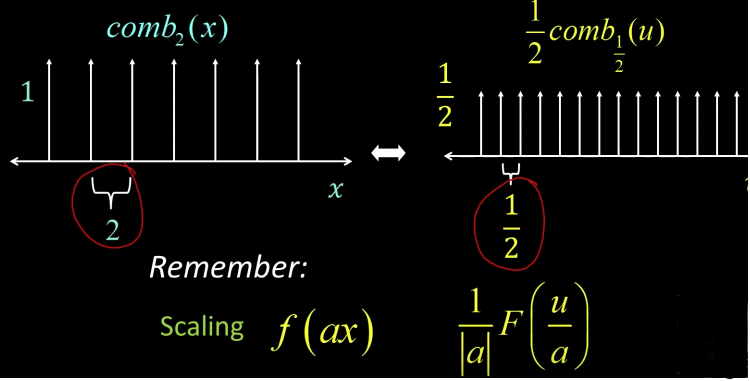
| Scaling | $$f(ax)$$ | Shrink<---->Stretch | $$\frac{1}{|a|}F(\frac{u}{a})$$ |
| Differentiation | $$\frac{d^nf(x)}{dx^n}$$ | $$(i2\pi u)''F(u)$$ |
Fourier Pairs
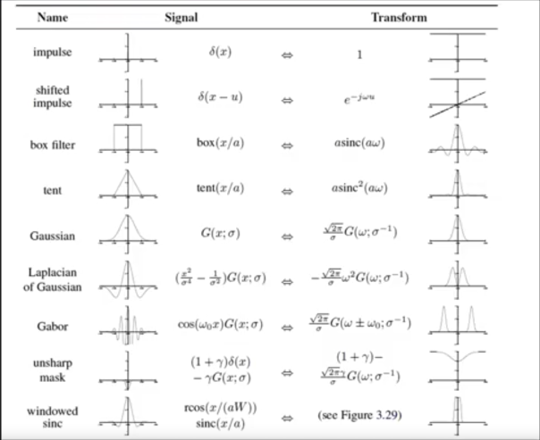
Fourier Transform Sampling Pairs
A fourier transform of pulse train is another pulse train.
A pulse train is comb function in the form
$$\sum_{n=-\infty}^{\infty}\delta(x-nx_0) $$
and its transform function is
$$\frac{1}{x_0}\sum_{n=-\infty}^{\infty}\delta(\epsilon-\frac{n}{x_0}) $$

%matplotlib inline
sin = lambda t,k,A,phi: + A*np.sin(2*np.pi*k*t + phi)
x = np.linspace(np.pi, 2*np.pi, 1000)
y = [sin(xi,2,1,0) for xi in x]
sampled = [y[i] for i in range(0,1000,10)]
fig,ax = plt.subplots(2,1)
fig.set_size_inches(8,8)
ax[0].plot(y)
ax[0].set_title("Continuous")
ax[1].bar(np.arange(len(sampled)),sampled)
ax[1].set_title("Sampled")

Reconstructing
- Making samples back into a continuous function
- for output (need realizable method)
- for analysis or processing (need mathematical)
- Amounts to "guessing" what the function did between
fig,ax = plt.subplots(2,1)
fig.set_size_inches(8,8)
ax[0].bar(np.arange(len(sampled)),sampled)
ax[0].set_title("Sampled")
ax[1].plot(sampled)
ax[1].set_title("Continous")

Example Audio
chirp
sin = lambda t,k,A,phi: + A*np.sin(2*np.pi*k*t + phi)
x = np.linspace(np.pi, 2*np.pi, 3000)
chirp = [sin(xi,5,1,0) for xi in x[:1000]] + [sin(xi,10,1,0) for xi in x[1000:2000]] + [sin(xi,15,1,0) for xi in x[2000:3000]]
plt.plot(chirp)

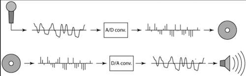
Sampling in digital audio
- Recording: sound to analog to samples to disk
- Playback: disk to samples to analog to sound again
undersampling
- Unsurprising results: information is lost
- Surprising results: indistinguishable from lower frequency (not shown below because plots are not smooth)
%matplotlib inline
sin = lambda t,k,A,phi: + A*np.sin(2*np.pi*k*t + phi)
x = np.linspace(np.pi, 2*np.pi, 1000)
y = [sin(xi,2,1,0) for xi in x]
fig,ax = plt.subplots(5,1)
fig.set_size_inches(8,20)
ax[0].plot(y)
ax[0].set_title("Continuous")
ax[1].plot([y[i] for i in range(0,1000,10)])
ax[1].set_title("Sampled every 10")
ax[2].plot([y[i] for i in range(0,1000,25)])
ax[2].set_title("Sampled every 25")
ax[3].plot([y[i] for i in range(0,1000,50)])
ax[3].set_title("Sampled every 50")
ax[4].plot([y[i] for i in range(0,1000,100)])
ax[4].set_title("Sampled every 100")

**Aliasing:** signals "traveling in disguise" as other frequencies
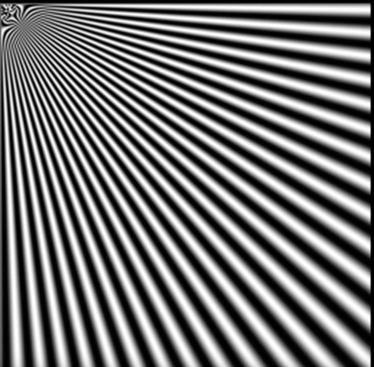
Aliasing in images

- The checkboard supposed to get thinner and closer as we move further, but at the far end it breaks up. This is aliasing where samples is not enough to reconstruct the signal
chirp = lambda x: np.sin((2**x)*x)
x = np.arange(0,5,0.009)
y = np.array([chirp(xi) for xi in x])
fig,ax = plt.subplots(2,1)
fig.set_size_inches(20,10)
ax[0].plot(y)
ax[0].set_title("Input Signal")
ax[1].imshow(np.array([y]*200))
ax[1].set_title("Plot as image")

Notice at the end where the frequecncy gets really high, there are no enough samples to reconstruct the correct signal and thus we see aliasing
Antialiasing (prevent aliasing)
- Sample more often
- Join the Mega-Pixel craze of the photo industry
- But this can't go on forever
- Make the signal less "wiggly"
- Get rid of some high frequencies
- Will lose information
- But it's better than aliasing
For instance, in audio decoding and encoding, to prevent aliasing, we can introduce lowpass filters:
- Remove high frequencies leaving only safe, low frequencies to be reconstructed

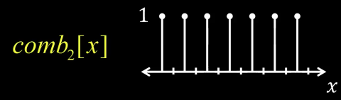
Impulse Train
Define a comb function (impulse train) in 1D as follows
$$ comb_M[x] = \sum_{k=-\infty}^{\infty}\delta[x - kM]$$
where $M$ is an integer, and $\delta$ function is a function that is 1 when its argument is zero and 0 otherwise. What this function means is that as k goes from minus infinity to infinity, x every M would be a one. So if $M$ is 2, than every 2 there is a one like below
FT of Impulse Train in 1D
Impulse in 2D (bed of nails)
$$ comb_{M,N}(x,y) = \sum_{k=-\infty}^{\infty}\sum_{l=-\infty}^{\infty}\delta(x-kM, y-lN)$$
The Fourier Transform of an impulse train is also an impulse train
$$ comb_{\frac{1}{M},\frac{1}{N}}(u,v) = \sum_{k=-\infty}^{\infty}\sum_{l=-\infty}^{\infty}\delta(u-\frac{k}{M},v-\frac{l}{N})$$
As the comb samples get further apart, the spectrum samples get closer together
Sampling low frequency signal

Sampling is just the multiplication of the signal with a comb function in the spatial domain. And in the frequency domain it is the convolvement with the comb function
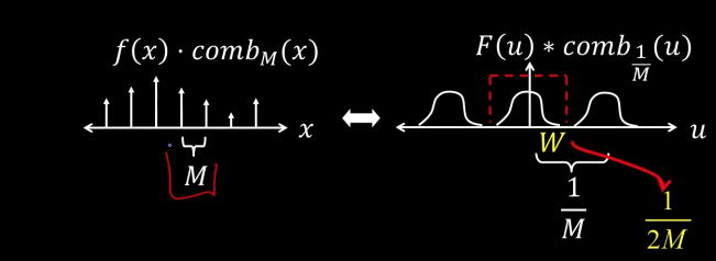
If the maximum frequency of the signal is small enough, than we can use one cone of the comb function to reconstruct the signal
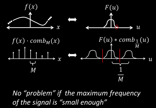
If the maximum frequency $W$ is less than $\frac{1}{2M}$, the original signal can be recovered from its samples by low-pass filtering
from scipy import signal
time_step = 0.02
period = 1.
x = np.arange(0, 20, time_step)
y = np.sin(2 * np.pi / period * x)
fig,ax = plt.subplots(3,1)
fig.set_size_inches(20,10)
ax[0].plot(y)
ax[0].set_title("Input Signal")
spacing = 4
comb = np.tile(signal.unit_impulse(spacing,spacing-1),int(y.size/spacing))
ax[1].stem(np.arange(30),comb[:30])
ax[1].set_title("Comb")
mul = y*comb
ax[2].plot(mul)
ax[2].set_title("Sampled")

from scipy.fftpack import fft, ifft
from scipy import signal
from scipy.signal import fftconvolve
from scipy.fftpack import fft
fig,ax = plt.subplots(3,2)
fig.set_size_inches(20,25)
Fs = 1000.0 # Sampling frequency
T = 1.0/Fs # Sampling period
L = 1500 # Length of signal
t = np.arange(0,(L)*T,T) # Time vector
S = 0.7*np.sin(2*np.pi*2*t)
ax[0,0].plot(S)
yf = fft(S)
xf = np.linspace(0.0, 1.0/(2.0*T), int(L/2))
ax[0,1].plot(t[:L//2], 2.0/L * np.abs(yf[:L//2]))
Tc = 30
comb = np.tile(signal.unit_impulse(Tc),L//Tc)
ax[1,0].stem(t,comb)
combfft = Tc*fft(comb)/L
ax[1,1].stem(t,np.abs(combfft))
ax[2,0].plot(S*comb)
conv = np.convolve(yf,combfft,mode='same')
# y = np.zeros(L)
# y[0:9] = np.abs(conv[0:9])
# iconv = ifft(y)
ax[2,1].plot(t, 2.0/L * np.abs(conv))


fig,ax = plt.subplots(3,2)
fig.set_size_inches(20,25)
S = 0.7*np.sin(70*np.pi*2*t) + 0.7*np.sin(5*np.pi*2*t)
ax[0,0].plot(S)
yf = fft(S)
xf = np.linspace(0.0, 1.0/(2.0*T), int(L/2))
ax[0,1].plot(t[:L//2], 2.0/L * np.abs(yf[:L//2]))
ax[1,0].stem(t,comb)
ax[1,1].stem(t,np.abs(combfft))
ax[2,0].plot(S*comb)
conv = np.convolve(yf,combfft,mode='same')
ax[2,1].plot(t[L//2-100:L//2+100], 2.0/L * np.abs(conv[L//2-100:L//2+100]))

So to fix, we can filter the high frequency, so we don't get an overlab

### This is from
### https://scipy-cookbook.readthedocs.io/items/SignalSmooth.html
def smooth(x,window_len=11,window='hanning'):
if x.ndim != 1:
raise (ValueError, "smooth only accepts 1 dimension arrays.")
if x.size < window_len:
raise (ValueError, "Input vector needs to be bigger than window size.")
if window_len<3:
return x
if not window in ['flat', 'hanning', 'hamming', 'bartlett', 'blackman']:
raise (ValueError, "Window is on of 'flat', 'hanning', 'hamming', 'bartlett', 'blackman'")
s=np.r_[x[window_len-1:0:-1],x,x[-2:-window_len-1:-1]]
#print(len(s))
if window == 'flat': #moving average
w=np.ones(window_len,'d')
else:
w=eval('np.'+window+'(window_len)')
y=np.convolve(w/w.sum(),s,mode='valid')
return y
swindow = 101
fig,ax = plt.subplots(4,2)
fig.set_size_inches(20,25)
S = 0.7*np.sin(70*np.pi*2*t) + 0.7*np.sin(5*np.pi*2*t)
ax[0,0].plot(S)
yf = fft(S)
xf = np.linspace(0.0, 1.0/(2.0*T), int(L/2))
ax[0,1].plot(t[:L//2], 2.0/L * np.abs(yf[:L//2]))
S = smooth(S,swindow)[swindow-1:-swindow]
ax[1,0].plot(S)
yf = fft(S)
xf = np.linspace(0.0, 1.0/(2.0*T), int(L/2))
ax[1,1].plot(t[:L//2], 2.0/L * np.abs(yf[:L//2]))
ax[2,0].stem(t,comb)
ax[2,1].stem(t,np.abs(combfft))
ax[3,0].plot(S*comb[:-swindow])
conv = np.convolve(yf,combfft[:-swindow],mode='same')
ax[3,1].plot(t[L//2-100:L//2+100], 2.0/L * np.abs(conv[L//2-100:L//2+100]))

imshow(messi)
imshow(messi[::2,::2])
imshow(messi[::4,::4])
imshow(messi[::8,::8])


## To see how bad subsampling is. The effect of aliasing
imshow(messi)
imshow(resize(messi[::2,::2],(messi.shape[1],messi.shape[0])))
imshow(resize(messi[::4,::4],(messi.shape[1],messi.shape[0])))
imshow(resize(messi[::8,::8],(messi.shape[1],messi.shape[0])))


Gaussian (lowpass) pre-filtering
Filter the image and then subsample
from skimage.filters import gaussian as gaussian_filter
imshow(messi)
print("Subsampling without antialiasing")
imshow(resize(messi[::8,::8],(messi.shape[1],messi.shape[0])))
gimg = messi.copy()
for i in range(3):
gimg = normalize_img(gaussian_filter(gimg, sigma=2,multichannel=True)).astype(np.uint8)
gimg = gimg[::2,::2]
print("Subsampling after antialiasing")
imshow(resize(gimg,(messi.shape[1],messi.shape[0])))
